LEAIC Learning Guide (SPSS): Using the LEAIC
Overview and General Approach
In this example, we will examine homicide rates. From the FBI’s website we can find the overall U.S. homicide rate (4.5 per 100,000 persons in 2013), and we can find rates for states, counties and even some cities. Homicide rates, expressed as a number of homicides (numerator) per 100,000 persons in a geographic region (denominator), are much more informative than raw counts. However, a rate for the U.S., a state, or even a city only tells us so much. What if we wanted to examine whether homicide is predominantly a male or female phenomenon, whether homicides are more common in certain age groups, or whether there is much difference among the states? To examine this, we need population data organized by sex, age category, and state. This information is not available with UCR/NIBRS data, but it is available with Census Bureau data. We will link these sources and examine the results.
To calculate rates, we need numerators and denominators. For our numerators we will use NIBRS data where we have selected victims of homicide. For the denominators we will get data from the Census Bureau’s American Community Survey (ACS) by using the Census’ data table tool to create a table and export it as a comma-separated value (CSV) file. There are other sources for this data, but the ACS and American Fact Finder are readily available. We will read the CSV file into SPSS so that we can merge it with the NIBRS and LEAIC files.
UCR and NIBRS data are organized by law enforcement agency. Each record in a file refers to one law enforcement agency. An ORI code is an alphanumeric identifier assigned to law enforcement agencies by the FBI’s National Crime Information Center. A given law enforcement agency may have many ORI codes used for a variety of purposes. For our purpose, we are interested only in the ORI code associated with reporting crime information. In the UCR summary-reporting system the ORI code is a seven-character field. In NIBRS it is a nine-character field. The LEAIC file, which is also organized by law enforcement agency, contains both.
What you will need
We will collect the data together during this guide so you do not need to download it now.
Data:
- National Incident-Based Reporting System Extract Files, 2013 – Victim-Level File
- Law Enforcement Agency Identifiers Crosswalk, 2012
- Demographic data from the Census’ data table tool
Software:
- SPSS
In this learning guide, our general approach is:
- Create a numerator file
- Match NIBRS homicide victim records, which contain law enforcement agency information, to LEAIC records
- Aggregate the matched file to the desired geography
- Create a denominator file
- Use the Census’ data table tool to create a table with the necessary information aggregated to the desired geography
- Merge the NIBRS-LEAIC file with the table from the Census
- Calculate rates
- Examine results
Example Task: Calculating Homicide Victimization Rates
We will use the NIBRS Extract Files for 2013. This file is located on the National Archive of Criminal Justice Data website, meaning that you will need an account to be able to download this data. Accounts are free and you can register for one on the ICPSR website. The NIBRS file is ICPSR study #36121, and we want the DS2 Victim-Level File (data set number 2 – Victim-Level Extract File). On this study’s homepage, there are a number of datasets available to download within the Data & Documentation tab. Since we are going to load this file into SPSS using an SPSS Setup file, click ASCII + SPSS Setup in the DS2: Victim-Level File download area. Read and agree to the Terms of Use. Clicking ASCII + SPSS Setup will download a zip file called ICPSR_36121-V2.zip which has a number of folders and files inside it. Because the file is zipped, you may need software designed to open compressed, or zipped files. Within ICPSR_36121-V2.zip there is a folder called ICPSR_36121. Within that, the key folder is “DS0002” which contains the setup file (36121-0002-Setup.sps) and the data file (36121-0002-Data.txt).
Note: In this walkthrough, we will provide SPSS syntax on a step-by-step basis. The full code is available here
Read the NIBRS File into SPSS
You will need to use the Setup file to read the data file into SPSS. We will then save it as an SPSS file for use throughout this guide. Open SPSS and in the file menu, click File -> Open -> Syntax. Choose the file 36121-0002-Setup.sps and click Open. This opens up an SPSS Setup file, which is an instruction manual to SPSS for how to read the data file. There are two changes you need to make to this file. The first is to set your working directory. The working directory tells SPSS to look in a specified folder for each file that you mention. A good practice is to keep all of your needed files in a single folder and set that folder as the Working Directory. Throughout this guide, we act as if the files are within the Working Directory.
* An example working directory command would be
* cd 'C:Documents and SettingsResearchLEAIC'.
* Note that the above example is the path structure for
* a Windows machine, an example of a path structure on a
* Mac machine is below.
* cd 'Users/ICPSR/Desktop/Research/LEAIC'.


cd 'ENTER YOUR WORKING DIRECTORY HERE'.
You must copy the above line (after changing the part inside the quotation marks to your own working directory) into the Setup file BEFORE line 50. Make sure that both the data file and the Setup file are inside the working directory folder.
The other change is to edit line 50. The value in the quotation marks in line 50 tells SPSS the name of the file you want it to read. Right now, that file is called “data-filename”. We need to change this to the real name of the file, 36121-0002-Data.txt.
Line 50 currently looks like this:
FILE HANDLE DATA / NAME=”data-filename” LRECL=1003.
Change this to:
FILE HANDLE DATA / NAME=”36121-0002-Data.txt” LRECL=1003.
Once you have made these changes, click Run -> All. Reading the file into SPSS may take several minutes. When the bottom of the SPSS window says “IBM SPSS Statistics Processor is Ready,” it’s done running. SPSS will open the data file. Save it as an SPSS file for use throughout this guide. In File, click Save As and name the file da36121-0002.sav.
Note: For a more detailed guide to using SPSS Setup files to read text data files, see this ICPSR guide
Select NIBRS Variables
The NIBRS files are large. Once converted to SPSS, the file is approximately 5.5 GB. We do not need all the information included in it, so we’ll just keep the variables we need. Referring to the codebook helps identify what variables are needed.
ORI ORIGINATING AGENCY IDENTIFIER

BH007 CITY NAME

BH019 CURRENT POPULATION 1

BH023 CURRENT POPULATION 2

BH027 CURRENT POPULATION 3

BH031 CURRENT POPULATION 4

BH035 CURRENT POPULATION 5

V4007 UCR OFFENSE CODE 1

V4008 UCR OFFENSE CODE 2

V4009 UCR OFFENSE CODE 3

V4010 UCR OFFENSE CODE 4

V4011 UCR OFFENSE CODE 5

V4012 UCR OFFENSE CODE 6

V4013 UCR OFFENSE CODE 7

V4014 UCR OFFENSE CODE 8

V4015 UCR OFFENSE CODE 9

V4016 UCR OFFENSE CODE 10

V4018 AGE OF VICTIM

V4019 SEX OF VICTIM
ORI is necessary to link to the LEAIC.
BH007 – CITY NAME, while technically not necessary, is a useful descriptive variable. It will also be useful to verify that we merged this data with the LEAIC data correctly.
Variables BH019, BH023, BH027, BH031, and BH035 are five population variables. NIBRS recognizes that some cities may span more than one county. The five CURRENT POPULATION variables record the portion of the city population that is in each county. The vast majority of cities have all of their population in one county. However, there are a few hundred that have populations in multiple counties. There is no one total population variable in NIBRS. We’ll create that later.
NIBRS records up to 10 offenses per victim. The vast majority of victims experience one offense. However, to be complete we need to look at all possible offense variables. Variables V4007 to V4016 record the offenses that the victim experienced. As an aside, for single-victim crime incidents, what is recorded in variables V4007 to V4016 will be the same as what is recorded on the NIBRS offense records. For multiple-victim crime incidents, what is recorded in V4007 to V4016 is specific to an individual victim.
V4018 – AGE OF VICTIM and V4019 – SEX OF VICTIM are the demographic variables we are interested in.
You will notice that we did not choose a state variable. That may seem odd given we intend to aggregate to state level. We did not bother with a state variable at this point because we will pick up the state when we merge these data with the LEAIC.
Get Numerator Data
Below is the SPSS code to read in the NIBRS Victim Extract File and select the variables we need. To open a new syntax file (where you will paste and run the following code) click File -> New -> Syntax. Then copy the following code and run it by highlighting the code and clicking Run -> Selection.
* Read the NIBRS 2013 Victim Extract File.
* This file is large ~ 5.5 gigs.
* Reduce the file by selecting only the variables that are needed.
* Referring to the codebook helps identify what is necessary.
* Make sure to copy the period at end of this chunk (the line right
* after V4019)!

cd 'ENTER YOUR WORKING DIRECTORY HERE'.

get file = "da36121-0002.sav"
  /keep
  ORI
  BH007 BH019 BH023 BH027 BH031 BH035
  V4007 V4008 V4009 V4010 V4011 V4012 V4013 V4014 V4015 V4016
  V4018
  V4019
.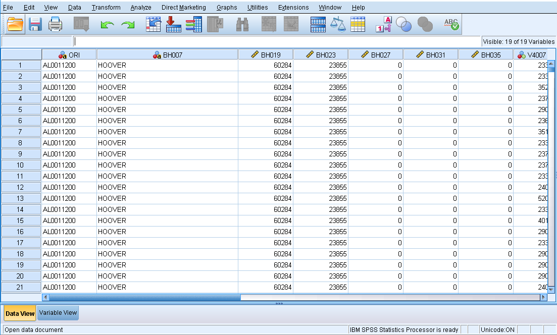
After running the above code, we have a file with 5,588,281 records – a record for each victim of crime in the NIBRS data. A window will open with the above table in Data View. The table may appear behind your syntax window, so try minimizing open windows if you don’t immediately see it. This table includes all crimes covered in NIBRS. Homicide is relatively rare, so we can greatly reduce the file by selecting just victims of homicide. The NIBRS data indicates which crime occurred by a code rather than the name of the crime (for a complete list of which codes correspond to which crimes, please see the codebook). The code for ‘homicide’ is ’91’. Remember that each victim may have up to 10 offenses recorded, so we will need to check all 10 of these offenses for homicide. It is convenient to create a flag variable to indicate that the record is one we are interested in.
* Further reduce the file size by selecting only the offense(s)
* that we are interested in.
*
* Create a variable to indicate if the offense of interest
* is recorded.
* Essentially, we are making a binary variable (0 or 1) to indicate if that
* victim was murdered (1 = murdered).


numeric OFFENSE.
variable labels OFFENSE "OFFENSE OF INTEREST".


* Consider all 10 UCR OFFENSE CODE variables to see if murder

* is in any of them.

if ( V4007 = 91  or
     V4008 = 91  or
     V4009 = 91  or
     V4010 = 91  or
     V4011 = 91  or
     V4012 = 91  or
     V4013 = 91  or
     V4014 = 91  or
     V4015 = 91  or
     V4016 = 91  )
     OFFENSE = 1
.


* Now select only victim records that had the offense of interest.

select if ( OFFENSE = 1 ).

* Create a frequency table to see how many murders there are in the data.

freq vars = OFFENSE.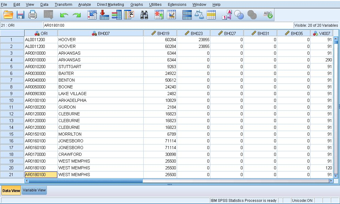
By creating a frequency table for the OFFENSE variable, we find that there are 3,551 victims of homicide in the NIBRS data. Remember, NIBRS does not include all of the United States, so this is just homicide victims recorded in NIBRS. If you look in the SPSS data editor you will see that each record has a code of 91 in one of the variables V4007 through V4016. You’ll also see that there are 3,551 records.
Now let’s create a total population variable. For our state-level analysis, that is all we need.
* Create a total population variable.

* There are five variables with population information so we will have to sum

* them all up to get the total population for each police agency.


numeric TOTPOP.
variable labels TOTPOP "TOTAL POPULATION".
compute TOTPOP = sum(BH019, BH023, BH027, BH031, BH035).
At this point we have a lot of variables that we do not need. Let’s sort the data by ORI and save a victim subset file keeping fewer variables.
* Sort and save this smaller file.

sort cases by ORI.
save outfile = "victim_subset.sav"
  /keep
  ORI
  BH007
  V4018
  V4019
 TOTPOP
 OFFENSE
.

get file = "victim_subset.sav"
.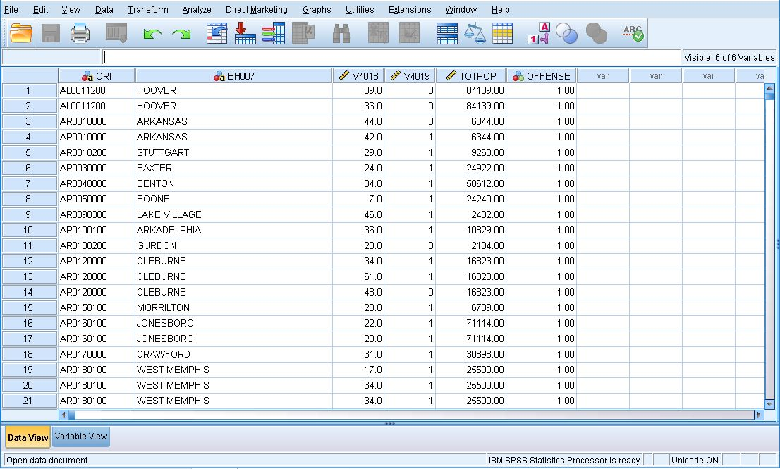
We now have a much smaller file than we started with. It’s much easier to work with and contains only what we are interested in. We sorted by ORI because that is what we will use to merge with the LEAIC. As you look at the individual records using the data editor notice that TOTPOP is repeated on each record having the same ORI code.
Get LEAIC Data
Now let’s get the data that we need from the LEAIC file. The LEAIC file is available to download in SPSS format from the study’s homepage, ICPSR study #35158. Under the Data & Documentation tab, click the button under Download and select SPSS (not “ASCII + SPSS Setup”). Agree to the Terms of Use and the file will begin to download. This file is a .sav file already so we do not need to use a Setup file to read it. Clicking SPSS will download a zipped folder called ICPSR_35158-V2.zip which contains a folder called ICPSR_35158. Within this folder is yet another folder called DS0001 which contains the file we want, 35158-0001-Data.sav (remember to move this file to your working directory).
We need the LEAIC file because the geography codes in the FBI’s UCR/NIBRS data are not the same as the codes used by the Census Bureau. The LEAIC has both sets of geography codes for each law enforcement agency. As with the NIBRS data, we don’t need all of the LEAIC variables or cases, so we’ll keep just what we need.
FSTATE FIPS STATE CODE
ORI9 ORIGINATING AGENCY IDENTIFIER (9 CHARACTERS)
NAME AGENCY NAME
FSTATE contains information on which state each agency is in. We will use this first to only select states where every agency reports to NIBRS and aggregate the crimes by state. Then we will use it to merge with the Census file. ORI9 is a nine-character long alphanumeric identifier that the FBI uses to identify each agency. Because NIBRS has an identical column, we will use it to merge the two data sets. NAME is the name of the agency and can be used to check that the crosswalk merged with the NIBRS file correctly. If the name of the agency is the same in NAME and BH007 (NIBRS column for the city name), we can be confident the merge was successful.
* Read the LEAIC file and keep only the variables we are interested in.

get file = "35158-0001-Data.sav"
  /keep
  FSTATE
  FPLACE
  ORI9
  NAME
  U_TPOP
.
alter type ORI9(a9).


* Select only records that have a valid value for the ORI9 code.
* This is important because after selection we will have a file
* with unique values for the ORIGINATING AGENCY IDENTIFIER.

select if ( ORI9 ne '-1' ).


* Sort the file by ORI9 and save a subset of the LEAIC.
sort cases by ORI9.
save outfile = "leaic_subset.sav".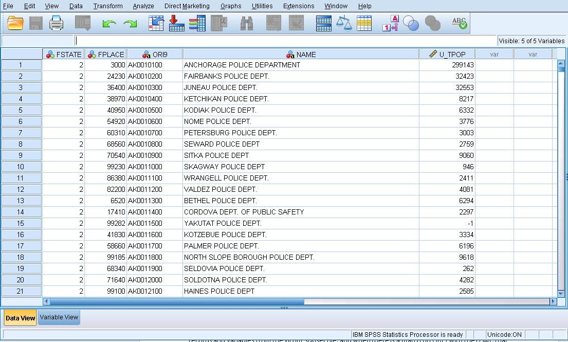
Merge NIBRS with LEAIC
Now it is time to merge our two subset files together. We merge the files using the ORI variable. In the NIBRS data the variable is simply named ORI. In the LEAIC file there are two ORI variables: a 7-character version and a 9-character version. We have to rename ORI in the NIBRS data to be compatible with the LEAIC. In the match files statement, the NIBRS data is referred to as “file” and the LEAIC data is referred to as “table”. What this means is that all the records from the file will be used, but only the data in the table that matches to the file will be included. Thus, our merged file will have all the records and variables from the victim subset file, and when there is a match on ORI9 with the LEAIC, that data will be included. We run a cross tabulation to get a summary of homicides by state.
* Merge the two subset files together.
* Use a 'table' match so that only records in the LEAIC subset that
* match to the victim subset are included.

match files
  /file = "victim_subset.sav"
  /rename (ORI = ORI9)
  /table = "leaic_subset.sav"
  /by ORI9
.


* Run a crosstabulation to see what we have -
* FIPS STATE CODE BY SEX OF VICTIM.

crosstabs /tables = FSTATE by V4019 /missing=include.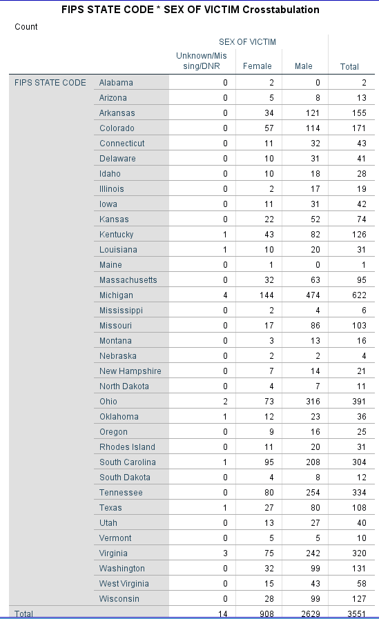
When we look at the cross tabulation output, we notice a few things: Data are not perfect. Remember that not all states participate in NIBRS, and of the ones that do, not all law enforcement agencies are included. However, some states, such as Michigan, are 100% NIBRS. There are also some missing data; the sex of the victim is unknown for 14 victims.
Looking at the individual records in the data editor we see what appears to be duplicate information. The names of the law enforcement agency and the populations are listed twice. For all the previous talk about keeping only what is necessary, why include this information twice? The reason is to help verify that the merge was done correctly. If we saw that variable BH007 (from NIBRS) contains DETROIT, but variable NAME (from LEAIC) contains ANN ARBOR, then something is wrong. This is simply a check to make sure that the merge worked correctly. If the names are the same, we can be confident our merge was successful. Visually inspecting the data shows us that the merge worked as expected. The population variable TOTPOP (from NIBRS) differs from the variable U_TPOP (from LEAIC) in most cases. This is because our NIBRS data is from 2013 while the LEAIC is from 2012. We will use population data from the Census, so don’t worry about this.
* Save a copy of our file (nl -> NIBRS-LEAIC).
save outfile = "nl_subset.sav".
Calculate Numerators
The file that we just saved has all we need to calculate the numerator portion of our homicide rates. We need to create state totals from the individual law enforcement records that we currently have. In SPSS we make use of the “aggregate” command. However, the first thing we need to do is make age category variables.
The NIBRS victim data includes the sex and age (in years) of the victims. We could calculate a victimization rate for every age, but people usually find rates for specific important ages and age categories more useful. We also need to be aware that our denominator data may not be in the same form as the numerator data. For instance, the ACS data we will get from the Census’ data table tool are not in the same form as the NIBRS data. Most age groups are categorized into 5-year categories (25-29, 30-34, etc.), but finer categories are used for ages 15-24, as those are the prime ages of criminal offending. The youngest and the oldest categories are grouped as ‘under 5 years’ and ’85 years and older’, respectively. We’ll make our numerator data – sex and victim age categories – match the denominator data from the ACS.
The ACS age categories are as follows:
| Under 5 years |
| 5 to 9 years |
| 10 to 14 years |
| 15 to 19 years |
| 20 to 24 years |
| 25 to 29 years |
| 30 to 34 years |
| 35 to 39 years |
| 40 to 44 years |
| 45 to 49 years |
| 50 to 54 years |
| 55 to 59 years |
| 60 to 64 years |
| 65 to 69 years |
| 70 to 74 years |
| 75 to 79 years |
| 80 to 84 years |
| 85 years and older |
The ACS data has 18 age categories for both females and males. The code below creates and labels 36 variables.
get file = "nl_subset.sav".

* Create SEX-AGE categories.
* V4018 (age), and V4019 (sex) of victim respectively.
* A nested DO-IF statement creates the category variables.
* The compute statements will create a value only if BOTH
* V4018 and V4019 have valid values.

DO IF ( V4019 = 0 ).
+ do if ( V4018 >= 0   and  V4018 < 5).
+ compute F_LT5 = 1.
+ else if ( V4018 >= 5   and  V4018 <= 9).
+ compute F5_9 = 1.
+ else if ( V4018 >= 10  and  V4018 <= 14 ).
+ compute F10_14 = 1.
+ else if ( V4018 >= 15  and  V4018 <= 19 ).
+ compute F15_19 = 1.
+ else if ( V4018 >= 20  and  V4018 <= 24 ).
+ compute F20_24 = 1.
+ else if ( V4018 >= 25  and  V4018 <= 29 ).
+ compute F25_29 = 1.
+ else if ( V4018 >= 30  and  V4018 <= 34 ).
+ compute F30_34 = 1.
+ else if ( V4018 >= 35  and  V4018 <= 39 ).
+ compute F35_39 = 1.
+ else if ( V4018 >= 40  and  V4018 <= 44 ).
+ compute F40_44 = 1.
+ else if ( V4018 >= 45  and  V4018 <= 49 ).
+ compute F45_49 = 1.
+ else if ( V4018 >= 50  and  V4018 <= 54 ).
+ compute F50_54 = 1.
+ else if ( V4018 >= 55  and  V4018 <= 59 ).
+ compute F55_59 = 1.
+ else if ( V4018 >= 60  and  V4018 <= 64 ).
+ compute F60_64 = 1.
+ else if ( V4018 >= 65  and  V4018 <= 69 ).
+ compute F65_69 = 1.
+ else if ( V4018 >= 70  and  V4018 <= 74 ).
+ compute F70_74 = 1.
+ else if ( V4018 >= 75  and  V4018 <= 79 ).
+ compute F75_79 = 1.
+ else if ( V4018 >= 80  and  V4018 <= 84 ).
+ compute F80_84 = 1.
+ else if ( V4018 >= 85 ).
+ compute F85_OVR = 1.
+ end if.
ELSE IF ( V4019 = 1 ).
+ do if ( V4018 >= 0   and  V4018 < 5).
+ compute M_LT5 = 1.
+ else if ( V4018 >= 5   and  V4018 <= 9).
+ compute M5_9 = 1.
+ else if ( V4018 >= 10  and  V4018 <= 14 ).
+ compute M10_14 = 1.
+ else if ( V4018 >= 15  and  V4018 <= 19 ).
+ compute M15_19 = 1.
+ else if ( V4018 >= 20  and  V4018 <= 24 ).
+ compute M20_24 = 1.
+ else if ( V4018 >= 25  and  V4018 <= 29 ).
+ compute M25_29 = 1.
+ else if ( V4018 >= 30  and  V4018 <= 34 ).
+ compute M30_34 = 1.
+ else if ( V4018 >= 35  and  V4018 <= 39 ).
+ compute M35_39 = 1.
+ else if ( V4018 >= 40  and  V4018 <= 44 ).
+ compute M40_44 = 1.
+ else if ( V4018 >= 45  and  V4018 <= 49 ).
+ compute M45_49 = 1.
+ else if ( V4018 >= 50  and  V4018 <= 54 ).
+ compute M50_54 = 1.
+ else if ( V4018 >= 55  and  V4018 <= 59 ).
+ compute M55_59 = 1.
+ else if ( V4018 >= 60  and  V4018 <= 64 ).
+ compute M60_64 = 1.
+ else if ( V4018 >= 65  and  V4018 <= 69 ).
+ compute M65_69 = 1.
+ else if ( V4018 >= 70  and  V4018 <= 74 ).
+ compute M70_74 = 1.
+ else if ( V4018 >= 75  and  V4018 <= 79 ).
+ compute M75_79 = 1.
+ else if ( V4018 >= 80  and  V4018 <= 84 ).
+ compute M80_84 = 1.
+ else if ( V4018 >= 85 ).
+ compute M85_OVR = 1.
+ end if.
END IF.


VARIABLE LABELS
  F_LT5           "FEMALE VICTIM LESS THAN 5 YEARS OLD"
  F5_9            "FEMALE VICTIMS 5 TO 9 YEARS OLD"
  F10_14          "FEMALE VICTIMS 10 TO 14 YEARS OLD"
  F15_19          "FEMALE VICTIMS 15 TO 19 YEARS OLD"
  F20_24          "FEMALE VICTIMS 20 TO 24 YEARS OLD"
  F25_29          "FEMALE VICTIMS 25 TO 29 YEARS OLD"
  F30_34          "FEMALE VICTIMS 30 TO 34 YEARS OLD"
  F35_39          "FEMALE VICTIMS 35 TO 39 YEARS OLD"
  F40_44          "FEMALE VICTIMS 40 TO 44 YEARS OLD"
  F45_49          "FEMALE VICTIMS 45 TO 49 YEARS OLD"
  F50_54          "FEMALE VICTIMS 50 TO 54 YEARS OLD"
  F55_59          "FEMALE VICTIMS 55 TO 59 YEARS OLD"
  F60_64          "FEMALE VICTIMS 60 TO 64 YEARS OLD"
  F65_69          "FEMALE VICTIMS 65 TO 69 YEARS OLD"
  F70_74          "FEMALE VICTIMS 70 TO 74 YEARS OLD"
  F75_79          "FEMALE VICTIMS 75 TO 79 YEARS OLD"
  F80_84          "FEMALE VICTIMS 80 TO 84 YEARS OLD"
  F85_OVR         "FEMALE VICTIMS 85 YEARS OLD AND OVER"

  M_LT5           "MALE VICTIM LESS THAN 5 YEARS OLD"
  M5_9            "MALE VICTIMS 5 TO 9 YEARS OLD"
  M10_14          "MALE VICTIMS 10 TO 14 YEARS OLD"
  M15_19          "MALE VICTIMS 15 TO 19 YEARS OLD"
  M20_24          "MALE VICTIMS 20 TO 24 YEARS OLD"
  M25_29          "MALE VICTIMS 25 TO 29 YEARS OLD"
  M30_34          "MALE VICTIMS 30 TO 34 YEARS OLD"
  M35_39          "MALE VICTIMS 35 TO 39 YEARS OLD"
  M40_44          "MALE VICTIMS 40 TO 44 YEARS OLD"
  M45_49          "MALE VICTIMS 45 TO 49 YEARS OLD"
  M50_54          "MALE VICTIMS 50 TO 54 YEARS OLD"
  M55_59          "MALE VICTIMS 55 TO 59 YEARS OLD"
  M60_64          "MALE VICTIMS 60 TO 64 YEARS OLD"
  M65_69          "MALE VICTIMS 65 TO 69 YEARS OLD"
  M70_74          "MALE VICTIMS 70 TO 74 YEARS OLD"
  M75_79          "MALE VICTIMS 75 TO 79 YEARS OLD"
  M80_84          "MALE VICTIMS 80 TO 84 YEARS OLD"
  M85_OVR         "MALE VICTIMS 85 YEARS OLD AND OVER"

.


* Run a frequency table before aggregating.
freq vars = FSTATE.
That is a lot of code, but remember we are interested in taking an overall rate – the U.S. homicide victimization rate – and looking at it in finer detail. That requires extra effort. Generating a frequency table for one variable – FSTATE – is sufficient to see that our code worked without errors. Working without error messages is not the same as working correctly. The frequency on FSTATE (FIPS STATE) already starts to tell us a more interesting story about homicide victims. We see a lot of variation among the states. That is to be expected given that states vary greatly in population, and we adjust for that later. We also see some numbers that, at first, make no sense. California is not listed at all, and Illinois shows 19 homicides. Remember that NIBRS does not currently include all states; California does not participate. Also, while the State of Illinois participates, the City of Chicago does not. We will select for states that are 100% NIBRS reporting soon.
Now it’s time to aggregate our sex-age category variables to get total counts. The aggregate command creates new variables that correspond to the total homicide victims by sex-age category. We also create variables for the total female, male and overall victim counts, and make labels for these new variables. We then select only the states that are 100% NIBRS reporting, which can be found on the FBI website. Finally, we recode system missing values to zero and save a file of victim counts. That file has all we need for our numerators.
* Aggregate to state totals.
aggregate outfile = *
  /break     =  FSTATE
  /TF_LT5    =  sum(F_LT5)
  /TF5_9     =  sum(F5_9)
  /TF10_14   =  sum(F10_14)
  /TF15_19   =  sum(F15_19)
  /TF20_24   =  sum(F20_24)
  /TF25_29   =  sum(F25_29)
  /TF30_34   =  sum(F30_34)
  /TF35_39   =  sum(F35_39)
  /TF40_44   =  sum(F40_44)
  /TF45_49   =  sum(F45_49)
  /TF50_54   =  sum(F50_54)
  /TF55_59   =  sum(F55_59)
  /TF60_64   =  sum(F60_64)
  /TF65_69   =  sum(F65_69)
  /TF70_74   =  sum(F70_74)
  /TF75_79   =  sum(F75_79)
  /TF80_84   =  sum(F80_84)
  /TF85_OVR  =  sum(F85_OVR)

  /TM_LT5    =  sum(M_LT5)
  /TM5_9     =  sum(M5_9)
  /TM10_14   =  sum(M10_14)
  /TM15_19   =  sum(M15_19)
  /TM20_24   =  sum(M20_24)
  /TM25_29   =  sum(M25_29)
  /TM30_34   =  sum(M30_34)
  /TM35_39   =  sum(M35_39)
  /TM40_44   =  sum(M40_44)
  /TM45_49   =  sum(M45_49)
  /TM50_54   =  sum(M50_54)
  /TM55_59   =  sum(M55_59)
  /TM60_64   =  sum(M60_64)
  /TM65_69   =  sum(M65_69)
  /TM70_74   =  sum(M70_74)
  /TM75_79   =  sum(M75_79)
  /TM80_84   =  sum(M80_84)
  /TM85_OVR  =  sum(M85_OVR)
.


compute TFEMALE  = sum(TF_LT5 to TF85_OVR).
compute TMALE    = sum(TM_LT5 to TM85_OVR).
compute TVICTIMS = sum(TFEMALE,TMALE).

* Add descriptive labels to these new variables.

VARIABLE LABELS
  TF_LT5     "TOTAL FEMALE VICTIMS LESS THAN 5 YEARS OLD"
  TF5_9      "TOTAL FEMALE VICTIMS 5 TO 9 YEARS OLD"
  TF10_14    "TOTAL FEMALE VICTIMS 10 TO 14 YEARS OLD"
  TF15_19    "TOTAL FEMALE VICTIMS 15 TO 19 YEARS OLD"
  TF20_24    "TOTAL FEMALE VICTIMS 20 TO 24 YEARS OLD"
  TF25_29    "TOTAL FEMALE VICTIMS 25 TO 29 YEARS OLD"
  TF30_34    "TOTAL FEMALE VICTIMS 30 TO 34 YEARS OLD"
  TF35_39    "TOTAL FEMALE VICTIMS 35 TO 39 YEARS OLD"
  TF40_44    "TOTAL FEMALE VICTIMS 40 TO 44 YEARS OLD"
  TF45_49    "TOTAL FEMALE VICTIMS 45 TO 49 YEARS OLD"
  TF50_54    "TOTAL FEMALE VICTIMS 50 TO 54 YEARS OLD"
  TF55_59    "TOTAL FEMALE VICTIMS 55 TO 59 YEARS OLD"
  TF60_64    "TOTAL FEMALE VICTIMS 60 TO 64 YEARS OLD"
  TF65_69    "TOTAL FEMALE VICTIMS 65 TO 69 YEARS OLD"
  TF70_74    "TOTAL FEMALE VICTIMS 70 TO 74 YEARS OLD"
  TF75_79    "TOTAL FEMALE VICTIMS 75 TO 79 YEARS OLD"
  TF80_84    "TOTAL FEMALE VICTIMS 80 TO 84 YEARS OLD"
  TF85_OVR   "TOTAL FEMALE VICTIMS 85 YEARS OLD AND OVER"
  TM_LT5     "TOTAL MALE VICTIMS LESS THAN 5 YEARS OLD"
  TM5_9      "TOTAL MALE VICTIMS 5 TO 9 YEARS OLD"
  TM10_14    "TOTAL MALE VICTIMS 10 TO 14 YEARS OLD"
  TM15_19    "TOTAL MALE VICTIMS 15 TO 19 YEARS OLD"
  TM20_24    "TOTAL MALE VICTIMS 20 TO 24 YEARS OLD"
  TM25_29    "TOTAL MALE VICTIMS 25 TO 29 YEARS OLD"
  TM30_34    "TOTAL MALE VICTIMS 30 TO 34 YEARS OLD"
  TM35_39    "TOTAL MALE VICTIMS 35 TO 39 YEARS OLD"
  TM40_44    "TOTAL MALE VICTIMS 40 TO 44 YEARS OLD"
  TM45_49    "TOTAL MALE VICTIMS 45 TO 49 YEARS OLD"
  TM50_54    "TOTAL MALE VICTIMS 50 TO 54 YEARS OLD"
  TM55_59    "TOTAL MALE VICTIMS 55 TO 59 YEARS OLD"
  TM60_64    "TOTAL MALE VICTIMS 60 TO 64 YEARS OLD"
  TM65_69    "TOTAL MALE VICTIMS 65 TO 69 YEARS OLD"
  TM70_74    "TOTAL MALE VICTIMS 70 TO 74 YEARS OLD"
  TM75_79    "TOTAL MALE VICTIMS 75 TO 79 YEARS OLD"
  TM80_84    "TOTAL MALE VICTIMS 80 TO 84 YEARS OLD"
  TM85_OVR   "TOTAL MALE VICTIMS 85 YEARS OLD AND OVER"
  TFEMALE    "TOTAL FEMALE VICTIMS"
  TMALE      "TOTAL MALE VICTIMS"
  TVICTIMS   "TOTAL VICTIMS"
.


* Select only states that are 100% NIBRS.

select if ( any(FSTATE,5,8,10,16,19,26,30,33,38,45,46,47,50,51,54) ).

* Recode system missing to zero.

recode TF_LT5 to TVICTIMS ( sysmis = 0 ).

save outfile = "victim_counts.sav".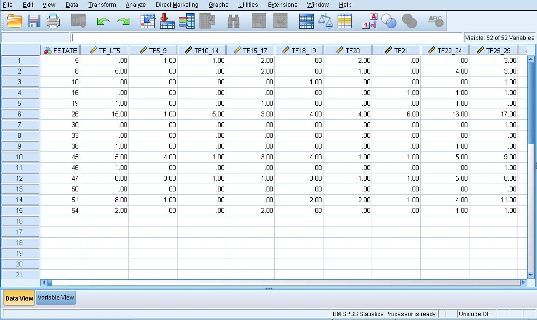
Note that sometimes after running code (for example, the above code), the data set will not visually change but will say “transformations pending” at the bottom of the window. This means that the code is working.
We’ve accomplished a lot. The file victim_counts.sav includes the homicide victim counts by sex-age category for each state that reports 100% NIBRS. We have our numerators. We are more than halfway to calculating disaggregated homicide victimization rates. The ACS data are already sex-age categorized, so we won’t have to repeat that work.
Calculate Denominators
We now have all the numerators needed for understanding homicide rates for different age and gender categories in NIBRS states. Now we must get the denominators. Since we want to look at crime rates in different population groups, we will use the Census’ ACS data to get the total number of people in each group. This will be our denominator.
There are a few ways to get Census data (e.g. using IPUMS which is an organization at the University of Minnesota that provides data from government surveys, including the Census), but we will find data using the Census’ data table tool. While the IPUMS gives raw data (or as close to raw as privacy concerns permit), the Census data table tool does some pre-processing for us. In our case that means that the data we retrieve will already be aggregated into the groups we want.
All data decisions in research come with trade-offs. The trade-off here is that our analysis is limited to the groups that the Census decided to provide. For example, whereas IPUMS provides age in years for all respondents (even in days for very young individuals), the Census provides age categories. A major benefit of the Census is that it aggregates the data for us. This reduces the amount of work we do ourselves and reduces the number of mistakes we can make. But it does restrict the number of categories of persons we can look at.
Is it important that we know the murder rate for women aged 72, or are we satisfied by the age category of 70-74? Does having more categories increase understanding without unnecessary complexity? The answer depends entirely on the question you are asking. As this guide is focused on using the LEAIC rather than Census data, this trade-off is acceptable to us. Your own research may necessitate more thorough data than the Census currently provides.
When conducting research, always consider the available data and how each data set can affect your research. Limitations in a data set mean limitations in your research. The very questions we can ask change based on the data we are using. Consider the data available and the questions you want to ask carefully before starting your research.
To get the necessary data from the Census data table tool, follow these steps:
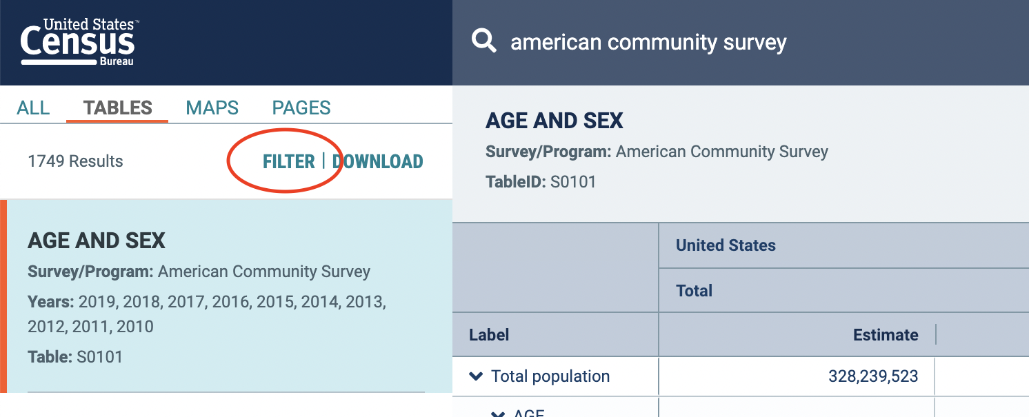
- Go to https://data.census.gov/
- In the search bar, search for “American Community Survey”
- Choose the first table that appears in the search results: “Age and Sex”
- After you click on the “Age and Sex” table, click the “Filter” button in the top left
- In the filter view, you will need to select the relevant data years and geography. Make sure you enter all of the following into the search bar: american community survey, 2013, Arkansas, Colorado, Delaware, Idaho, Iowa, Michigan, Montana, New Hampshire, North Dakota, South Carolina, South Dakota, Tennessee, Vermont, Virginia, West Virginia. This selection allows us to get only the 2013 data that we are interested in (the same year as our NIBRS data), as well as the 15 states that had 100% of agencies reporting to NIBRS in 2013.
- The 100% NIBRS states in 2013 are Arkansas, Colorado, Delaware, Idaho, Iowa, Michigan, Montana, New Hampshire, North Dakota, South Carolina, South Dakota, Tennessee, Vermont, Virginia, and West Virginia, the states we selected in our filter.
- Click Search.
- Finally, we need to select the data set to get the above variables from. When you are in your table view, you will find a “Product” dropdown in the top right corner. In the dropdown menu, select “2013: ACS 5-Year Estimates Subject Tables”.
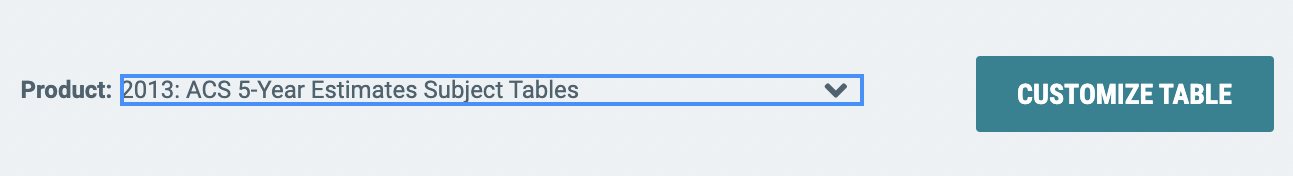
- 1-year estimates give data from the survey given that year. 3- and 5-year estimates use data from the selected year and the year before and after (or two years before and after for 5-year estimates). These two data sets have far more information than the 1-year estimate (due to covering more people in their combined surveys) but are less precise for the given year.
- As mentioned above, there are trade-offs with any data set. 1-year estimates only have data from the year in question, so are better able to answer questions about what is going on in that year. However, they do have fewer respondents than 3- or 5-year estimates. None of the data sets are objectively better than another (and this is true with nearly all data sets). You must first understand what information the data have available and determine if it can answer the questions you want to ask.
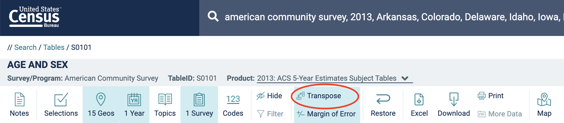
- We are done specifying what data we want. By default, our table has states as columns and age categories as rows. For easier analysis, let’s swap them. Click Customize Table and then Transpose:
- To download the data, click Download, select CSV format, and then uncheck the checkboxes that emerge. Click the Download button to download a zipped file containing the data.
- Downloading the data will open a folder with multiple files. The .csv file that you want includes “ACSST5Y2013.S0101_data_with_overlays” in the title. Move it to your working directory folder.
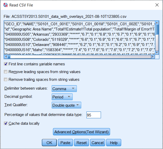
For simplicity we will read this Excel file into SPSS and save it as a SPSS file (file extension .sav). Open SPSS and in the File menu, go to Import Data and click CSV Data. From here you can navigate to the .csv file in your working directory and click Open. We need to do a bit of data prep with the ACS file. A Read CSV File window will open. Click Advanced Options(Text Wizard).
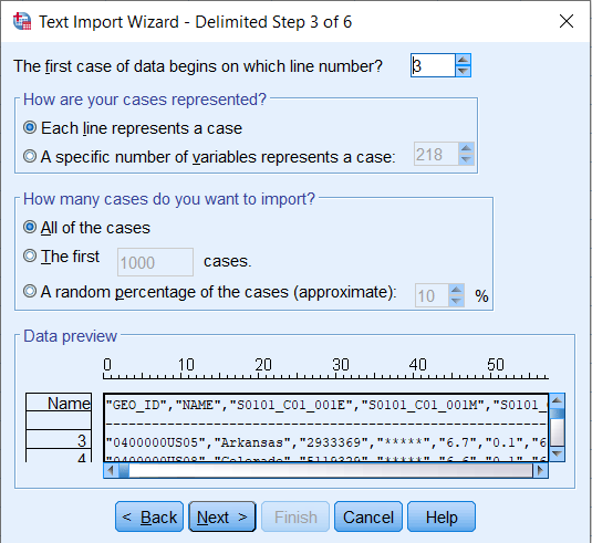
A Text Import Wizard – Step 1 of 6 window will open. Click Next for Steps 1 and 2 without making any changes. At Step 3, change the first dropdown box to 3. The CSV file contains label information in the first 2 rows, so the data first appear in row 3. Click Next.
Click Next for Step 4 without making any changes. Several changes are needed in Step 5. First, under Data preview, highlight the NAME column. In the Variable name box, change NAME to GEO.displaylabel.
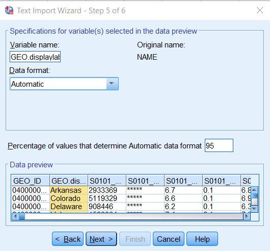
Go back under Data preview, highlight the third column, scroll all the way to the right, press SHIFT and highlight the last column to select all the variables in between. Under Data format, use the dropdown bar to select Numeric. These variables will be imported as strings otherwise. Click Next. (It’s okay that some variables have (X) values; they won’t be used.)

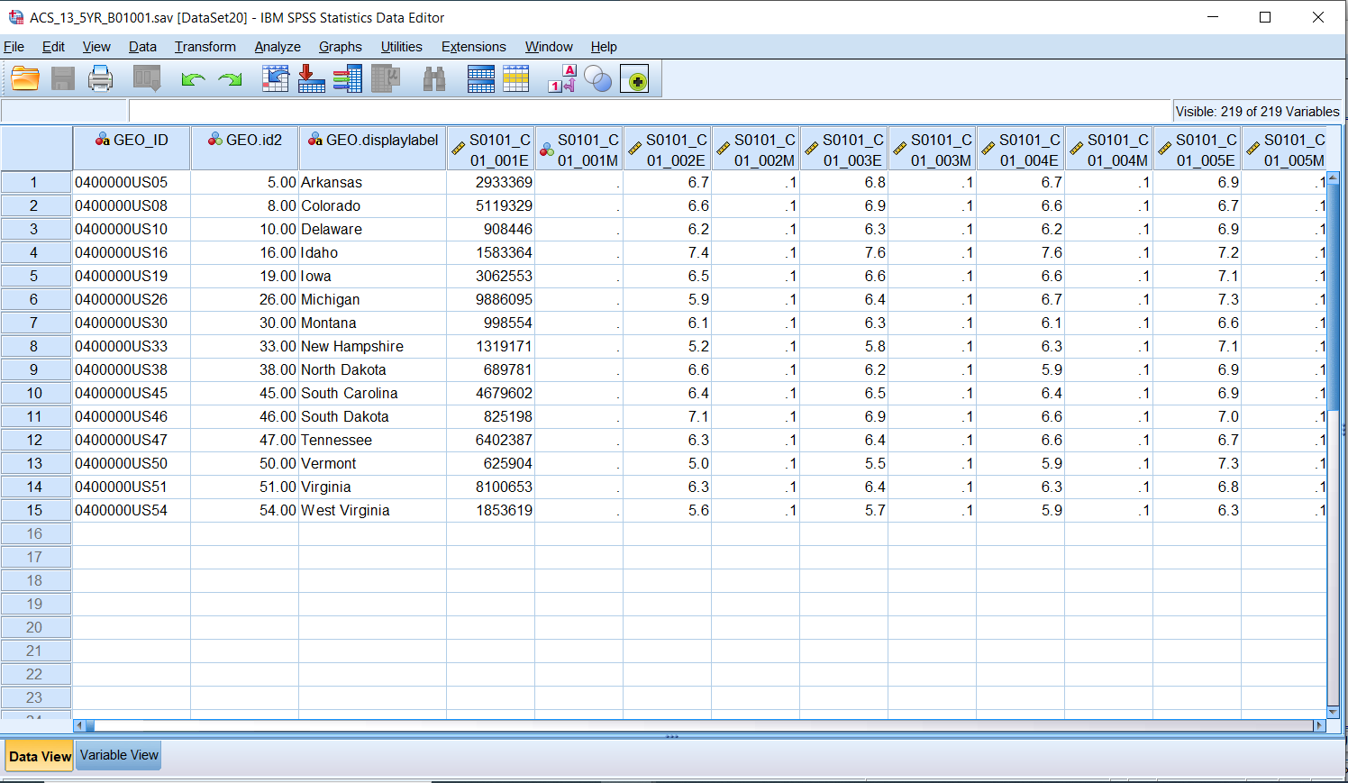
Click Finish at Step 6. The data should now be in an SPSS Data Editor window. Now save it as an SPSS file by clicking File -> Save As. The default file type is an SPSS file so simply name it ACS_13_5YR_B01001.sav and click Save. Move this file to your working directory.
Calculate Rates
Finally, we can combine our numerator and denominator files into one file and calculate disaggregated homicide rates. In the SPSS match files statement the victim counts are in the “file” statement. All records from that file will be included in the merged (matched) file. The ACS populations are referred to as a “table”. The ACS table includes population data for all states. Referring to it as a table means that only the records that match the “file” will be included in the resulting combined data file.
After the merge is done we calculate the homicide victimization rates by sex and age-category. The rate calculation is the number of homicide victims by sex and age category multiplied by 100,000 and divided by the number of persons in that sex and age category.
Our last data management task is to save our data. We save two files. One file has both rates and counts, which is useful for verification. The second has just the rates.
* * Create numeric version of GEO.id and combine the ACS population file with the victim counts file.

get file = "ACS_13_5YR_B01001.sav".

string GEO.idtemp (a2).
compute GEO.idtemp = char.substr(GEO_ID,10,2).
recode GEO.idtemp (convert) into GEO.id2.

save outfile = "ACS_13_5YR_B01001.sav"
  /keep=GEO_ID GEO.id2 GEO.displaylabel S0101_C01_001E to S0101_C03_036M.


match files
  /file = "victim_counts.sav"
  /table = "ACS_13_5YR_B01001.sav"
  /rename (GEO.id2 = FSTATE)
  /by FSTATE


* Calculate rates. The ACS data only provides percentages for each age
* category. We need to calculate the population totals for each age category.

* Example:
*   RTF_LT5,   rate of homicide victimization for females
*              less than 5 years old.
*   TF_LT5,    total count of female homicide victims
*              less than 5 years old.
*   S0101_C03_002E,    percentage of population of females
*              less than 5 years old per the American Community Survey.
*   S0101_C03_001E,    total population of females per
*              the American Community Survey.
*   POPF_LT5, the population of females less than
*              5 years old.

compute POPF_LT5 = (S0101_C03_002E/100)*S0101_C03_001E.
compute POPF5_9 = (S0101_C03_003E/100)*S0101_C03_001E.
compute POPF10_14 = (S0101_C03_004E/100)*S0101_C03_001E.
compute POPF15_19 = (S0101_C03_005E/100)*S0101_C03_001E.
compute POPF20_24 = (S0101_C03_006E/100)*S0101_C03_001E.
compute POPF25_29 = (S0101_C03_007E/100)*S0101_C03_001E.
compute POPF30_34 = (S0101_C03_008E/100)*S0101_C03_001E.
compute POPF35_39 = (S0101_C03_009E/100)*S0101_C03_001E.
compute POPF40_44 = (S0101_C03_010E/100)*S0101_C03_001E.
compute POPF45_49 = (S0101_C03_011E/100)*S0101_C03_001E.
compute POPF50_54 = (S0101_C03_012E/100)*S0101_C03_001E.
compute POPF55_59 = (S0101_C03_013E/100)*S0101_C03_001E.
compute POPF60_64 = (S0101_C03_014E/100)*S0101_C03_001E.
compute POPF65_69 = (S0101_C03_015E/100)*S0101_C03_001E.
compute POPF70_74 = (S0101_C03_016E/100)*S0101_C03_001E.
compute POPF75_79 = (S0101_C03_017E/100)*S0101_C03_001E.
compute POPF80_84 = (S0101_C03_018E/100)*S0101_C03_001E.
compute POPF85_OVR = (S0101_C03_019E/100)*S0101_C03_001E.

compute POPM_LT5 = (S0101_C02_002E/100)*S0101_C02_001E.
compute POPM5_9 = (S0101_C02_003E/100)*S0101_C02_001E.
compute POPM10_14 = (S0101_C02_004E/100)*S0101_C02_001E.
compute POPM15_19 = (S0101_C02_005E/100)*S0101_C02_001E.
compute POPM20_24 = (S0101_C02_006E/100)*S0101_C02_001E.
compute POPM25_29 = (S0101_C02_007E/100)*S0101_C02_001E.
compute POPM30_34 = (S0101_C02_008E/100)*S0101_C02_001E.
compute POPM35_39 = (S0101_C02_009E/100)*S0101_C02_001E.
compute POPM40_44 = (S0101_C02_010E/100)*S0101_C02_001E.
compute POPM45_49 = (S0101_C02_011E/100)*S0101_C02_001E.
compute POPM50_54 = (S0101_C02_012E/100)*S0101_C02_001E.
compute POPM55_59 = (S0101_C02_013E/100)*S0101_C02_001E.
compute POPM60_64 = (S0101_C02_014E/100)*S0101_C02_001E.
compute POPM65_69 = (S0101_C02_015E/100)*S0101_C02_001E.
compute POPM70_74 = (S0101_C02_016E/100)*S0101_C02_001E.
compute POPM75_79 = (S0101_C02_017E/100)*S0101_C02_001E.
compute POPM80_84 = (S0101_C02_018E/100)*S0101_C02_001E.
compute POPM85_OVR = (S0101_C02_019E/100)*S0101_C02_001E.

compute RTF_LT5 = 100000 * TF_LT5 / POPF_LT5.
compute RTF5_9 = 100000 * TF5_9 / POPF5_9.
compute RTF10_14 = 100000 * TF10_14 / POPF10_14.
compute RTF15_19 = 100000 * TF15_19 / POPF15_19.
compute RTF20_24 = 100000 * TF20_24 / POPF20_24.
compute RTF25_29 = 100000 * TF25_29 / POPF25_29.
compute RTF30_34 = 100000 * TF30_34 / POPF30_34.
compute RTF35_39 = 100000 * TF35_39 / POPF35_39.
compute RTF40_44 = 100000 * TF40_44 / POPF40_44.
compute RTF45_49 = 100000 * TF45_49 / POPF45_49.
compute RTF50_54 = 100000 * TF50_54 / POPF50_54.
compute RTF55_59 = 100000 * TF55_59 / POPF55_59.
compute RTF60_64 = 100000 * TF60_64 / POPF60_64.
compute RTF65_69 = 100000 * TF65_69 / POPF65_69.
compute RTF70_74 = 100000 * TF70_74 / POPF70_74.
compute RTF75_79 = 100000 * TF75_79 / POPF75_79.
compute RTF80_84 = 100000 * TF80_84 / POPF80_84.
compute RTF85_OVR = 100000 * TF85_OVR / POPF85_OVR.

compute RTM_LT5 = 100000 * TM_LT5 / POPM_LT5.
compute RTM5_9 = 100000 * TM5_9 / POPM5_9.
compute RTM10_14 = 100000 * TM10_14 / POPM10_14.
compute RTM15_19 = 100000 * TM15_19 / POPM15_19.
compute RTM20_24 = 100000 * TM20_24 / POPM20_24.
compute RTM25_29 = 100000 * TM25_29 / POPM25_29.
compute RTM30_34 = 100000 * TM30_34 / POPM30_34.
compute RTM35_39 = 100000 * TM35_39 / POPM35_39.
compute RTM40_44 = 100000 * TM40_44 / POPM40_44.
compute RTM45_49 = 100000 * TM45_49 / POPM45_49.
compute RTM50_54 = 100000 * TM50_54 / POPM50_54.
compute RTM55_59 = 100000 * TM55_59 / POPM55_59.
compute RTM60_64 = 100000 * TM60_64 / POPM60_64.
compute RTM65_69 = 100000 * TM65_69 / POPM65_69.
compute RTM70_74 = 100000 * TM70_74 / POPM70_74.
compute RTM75_79 = 100000 * TM75_79 / POPM75_79.
compute RTM80_84 = 100000 * TM80_84 / POPM80_84.
compute RTM85_OVR = 100000 * TM85_OVR / POPM85_OVR.

compute RTFEMALE       = 100000 * TFEMALE /S0101_C03_001E.
compute RTMALE         = 100000 * TMALE / S0101_C02_001E.

*** Add the female and male totals to get the population total.
compute ACSVICTIM = SUM(S0101_C03_001E,S0101_C02_001E).
compute RTVICTIMS      = 100000 * TVICTIMS / ACSVICTIM.

* Add descriptive labels to these new variables.
variable labels
  RTF_LT5    "HOMICIDE RATE ESTIMATE - FEMALE UNDER 5 YEARS"
  RTF5_9     "HOMICIDE RATE ESTIMATE - FEMALE 5 TO 9 YEARS"
  RTF10_14   "HOMICIDE RATE ESTIMATE - FEMALE 10 TO 14 YEARS"
  RTF15_19   "HOMICIDE RATE ESTIMATE - FEMALE 15 TO 19 YEARS"
  RTF20_24   "HOMICIDE RATE ESTIMATE - FEMALE 20 TO 24 YEARS"
  RTF25_29   "HOMICIDE RATE ESTIMATE - FEMALE 25 TO 29 YEARS"
  RTF30_34   "HOMICIDE RATE ESTIMATE - FEMALE 30 TO 34 YEARS"
  RTF35_39   "HOMICIDE RATE ESTIMATE - FEMALE 35 TO 39 YEARS"
  RTF40_44   "HOMICIDE RATE ESTIMATE - FEMALE 40 TO 44 YEARS"
  RTF45_49   "HOMICIDE RATE ESTIMATE - FEMALE 45 TO 49 YEARS"
  RTF50_54   "HOMICIDE RATE ESTIMATE - FEMALE 50 TO 54 YEARS"
  RTF55_59   "HOMICIDE RATE ESTIMATE - FEMALE 55 TO 59 YEARS"
  RTF60_64   "HOMICIDE RATE ESTIMATE - FEMALE 60 AND 64 YEARS"
  RTF65_69   "HOMICIDE RATE ESTIMATE - FEMALE 65 AND 69 YEARS"
  RTF70_74   "HOMICIDE RATE ESTIMATE - FEMALE 70 TO 74 YEARS"
  RTF75_79   "HOMICIDE RATE ESTIMATE - FEMALE 75 TO 79 YEARS"
  RTF80_84   "HOMICIDE RATE ESTIMATE - FEMALE 80 TO 84 YEARS"
  RTF85_OVR  "HOMICIDE RATE ESTIMATE - FEMALE 85 YEARS AND OVER"
  RTM_LT5    "HOMICIDE RATE ESTIMATE - MALE UNDER 5 YEARS"
  RTM5_9     "HOMICIDE RATE ESTIMATE - MALE 5 TO 9 YEARS"
  RTM10_14   "HOMICIDE RATE ESTIMATE - MALE 10 TO 14 YEARS"
  RTM15_19   "HOMICIDE RATE ESTIMATE - MALE 15 TO 19 YEARS"
  RTM20_24   "HOMICIDE RATE ESTIMATE - MALE 22 TO 24 YEARS"
  RTM25_29   "HOMICIDE RATE ESTIMATE - MALE 25 TO 29 YEARS"
  RTM30_34   "HOMICIDE RATE ESTIMATE - MALE 30 TO 34 YEARS"
  RTM35_39   "HOMICIDE RATE ESTIMATE - MALE 35 TO 39 YEARS"
  RTM40_44   "HOMICIDE RATE ESTIMATE - MALE 40 TO 44 YEARS"
  RTM45_49   "HOMICIDE RATE ESTIMATE - MALE 45 TO 49 YEARS"
  RTM50_54   "HOMICIDE RATE ESTIMATE - MALE 50 TO 54 YEARS"
  RTM55_59   "HOMICIDE RATE ESTIMATE - MALE 55 TO 59 YEARS"
  RTM60_64   "HOMICIDE RATE ESTIMATE - MALE 60 AND 64 YEARS"
  RTM65_69   "HOMICIDE RATE ESTIMATE - MALE 65 AND 69 YEARS"
  RTM70_74   "HOMICIDE RATE ESTIMATE - MALE 70 TO 74 YEARS"
  RTM75_79   "HOMICIDE RATE ESTIMATE - MALE 75 TO 79 YEARS"
  RTM80_84   "HOMICIDE RATE ESTIMATE - MALE 80 TO 84 YEARS"
  RTM85_OVR  "HOMICIDE RATE ESTIMATE - MALE 85 YEARS AND OVER"
  RTFEMALE   "HOMICIDE RATE ESTIMATE - FEMALE"
  RTMALE     "HOMICIDE RATE ESTIMATE - MALE"
  RTVICTIMS  "HOMICIDE RATE ESTIMATE - TOTAL"
.


* Set format for the new variables.

formats RTF_LT5 to RTVICTIMS (F5.1).


* Save two files: rates and counts and just rates.

save outfile = "rates_and_counts.sav"
  /keep
  FSTATE
  GEO.displaylabel
RTVICTIMS      TVICTIMS     ACSVICTIM
  RTFEMALE       TFEMALE      S0101_C03_001E
  RTMALE         TMALE        S0101_C02_001E
  RTF_LT5        TF_LT5       POPF_LT5
  RTF5_9         TF5_9        POPF5_9
  RTF10_14       TF10_14      POPF10_14
  RTF15_19       TF15_19      POPF15_19
  RTF20_24       TF20_24      POPF20_24
  RTF25_29       TF25_29      POPF25_29
  RTF30_34       TF30_34      POPF30_34
  RTF35_39       TF35_39      POPF35_39
  RTF40_44       TF40_44      POPF40_44
  RTF45_49       TF45_49      POPF45_49
  RTF50_54       TF50_54      POPF50_54
  RTF55_59       TF55_59      POPF55_59
  RTF60_64       TF60_64      POPF60_64
  RTF65_69       TF65_69      POPF65_69
  RTF70_74       TF70_74      POPF70_74
  RTF75_79       TF75_79      POPF75_79
  RTF80_84       TF80_84      POPF80_84
  RTF85_OVR      TF85_OVR     POPF85_OVR
  RTM_LT5        TM_LT5       POPM_LT5
  RTM5_9         TM5_9        POPM5_9
  RTM10_14       TM10_14      POPM10_14
  RTM15_19       TM15_19      POPM15_19
  RTM20_24       TM20_24      POPM20_24
  RTM25_29       TM25_29      POPM25_29
  RTM30_34       TM30_34      POPM30_34
  RTM35_39       TM35_39      POPM35_39
  RTM40_44       TM40_44      POPM40_44
  RTM45_49       TM45_49      POPM45_49
  RTM50_54       TM50_54      POPM50_54
  RTM55_59       TM55_59      POPM55_59
  RTM60_64       TM60_64      POPM60_64
  RTM65_69       TM65_69      POPM65_69
  RTM70_74       TM70_74      POPM70_74
  RTM75_79       TM75_79      POPM75_79
  RTM80_84       TM80_84      POPM80_84
  RTM85_OVR      TM85_OVR     POPM85_OVR.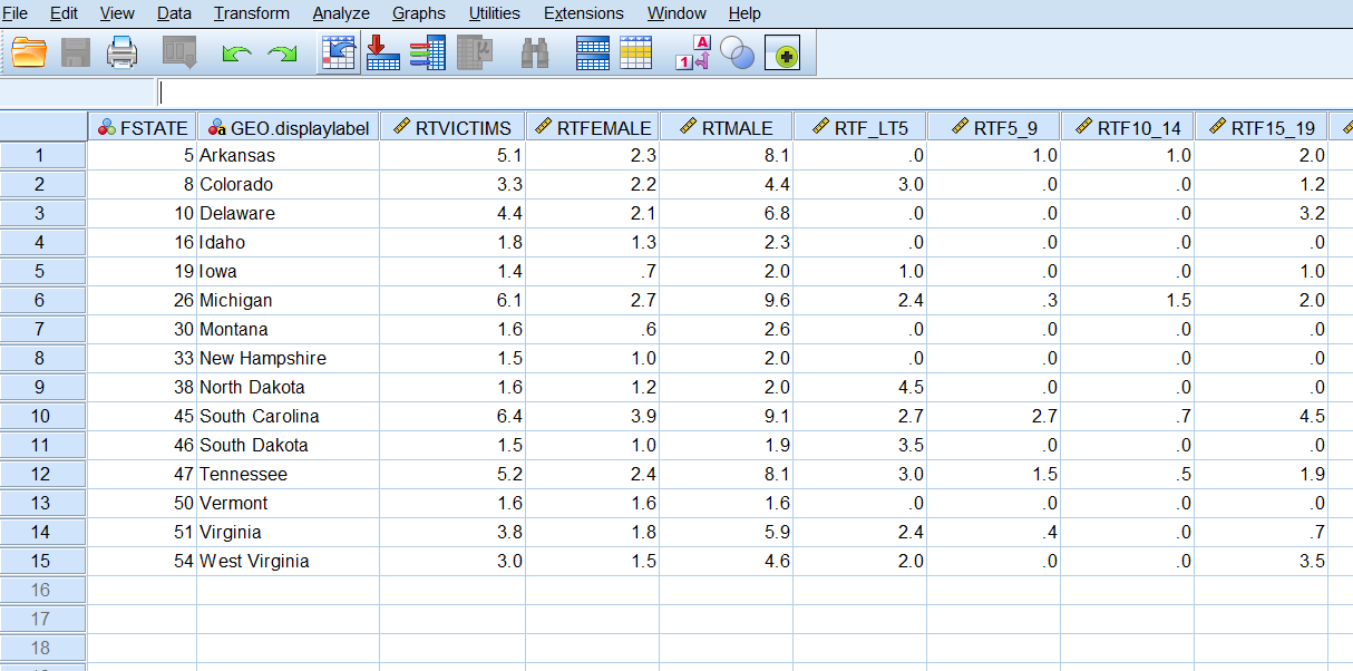
save outfile = "just_rates.sav"
  /keep
  FSTATE
  GEO.displaylabel
  RTVICTIMS
  RTFEMALE
  RTMALE
  RTF_LT5
  RTF5_9
  RTF10_14
  RTF15_19
  RTF20_24
  RTF25_29
  RTF30_34
  RTF35_39
  RTF40_44
  RTF45_49
  RTF50_54
  RTF55_59
  RTF60_61
  RTF62_64
  RTF65_66
  RTF67_69
  RTF70_74
  RTF75_79
  RTF80_84
  RTF85_OVR
  RTM_LT5
  RTM5_9
  RTM10_14
  RTM15_19
  RTM20_24
  RTM25_29
  RTM30_34
  RTM35_39
  RTM40_44
  RTM45_49
  RTM50_54
  RTM55_59
  RTM60_61
  RTM62_64
  RTM65_66
  RTM67_69
  RTM70_74
  RTM75_79
  RTM80_84
  RTM85_OVR
.
- Open these files to see your results. Click File -> Open -> Data, select the file you want, and click Open
You have now created files with the calculated homicide rates by sex and age category for the states participating 100% in NIBRS for the year 2013. Along the way we have used NIBRS, ACS, and LEAIC data; we’ve created subsets, merged files, computed new variables and aggregated variables; we tested the results of our work at key points; we calculated the disaggregated rates and saved our final files. We are now able to see how different the individual rates are from the overall U.S. rate that we started with.
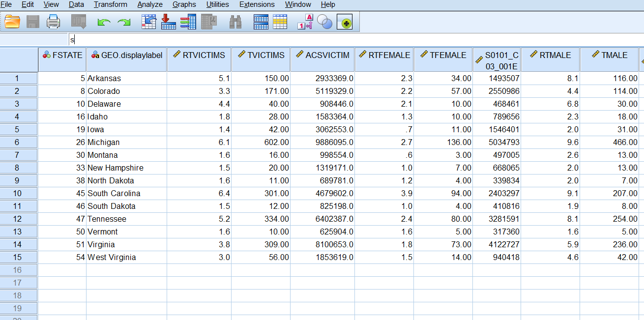
Examine the Results
If we use the data editor to examine individual values in the file just_rates.sav, we immediately see results that tell us much more than the overall U.S. homicide victimization rate. Total victimization rates by state vary from 1.4 (Iowa) to 6.4 (South Carolina). In each state, the homicide victimization rate for males is higher than for females, except in Vermont, where they are equal. These results are easy to see just by looking at the individual records.
Find the Highest Rates per State
The file just_rates.sav is not large. We could simply read across each row to find the age category with the largest rate in each state.
| STATE | RATE_CATEGORY | RATE |
|---|---|---|
| Arkansas | RTM30_34 | 22.4 |
| Colorado | RTM20_24 | 10.1 |
| Delaware | RTM15_19 | 25.3 |
| Idaho | RTM85_OVR | 10.5 |
| Iowa | RTM20_24 | 7.1 |
| Michigan | RTM25_29 | 25.7 |
| Montana | RTM40_44 | 10.3 |
| New Hampshire | RTM80_84 | 9.6 |
| North Dakota | RTM30_34 | 12.8 |
| South Carolina | RTM20_24 | 21.1 |
| South Dakota | RTM_LT5 | 9.9 |
| Tennessee | RTM25_29 | 22.8 |
| Vermont | RTF70_74 | 17.5 |
| Virginia | RTM20_24 | 12.8 |
| West Virginia | RTM25_29 | 16.7 |
Are the results surprising? For the most part we see relatively young males as victims. But what is going on with Idaho, New Hampshire, and Vermont? In Vermont, Females 70 to 74 years old have the highest homicide victimization rate in the state. Can this be correct? The answer is yes, but it is worth looking into why it is correct.
Vermont is a relatively low population state. Consequently, a single homicide can substantially affect their homicide rate. In addition, since we are looking at disaggregated rates, the denominator we use is small, which magnifies the effect. Looking at the file we just created – rates_and_counts.sav – we see that the population of females aged 70 to 74 in Vermont is only 11,425 (POPF70_74), and there are two female victims of homicide in this age group. The rate of 17.5 (RTF70_74) is simply ( 2 * 100,000 ) /11,425. The rate is correct, but we should be careful given how sensitive it is to change. One less homicide cuts the rate in half, and one more increases it by 50%.
Programmatically Find the Highest Rates per State
Visually inspecting a file this size is not too burdensome. However, when all states are 100% NIBRS, visual inspection could be tedious and prone to error. Below is SPSS code to produce a table identifying the sex-age categories with the highest rates.
* Read the file of rates.

get file = "just_rates.sav".


* The varstocases command transposes certain variables
* into cases and creates two new variables that can
* be analyzed.

varstocases
  /make RATE_PER_CAT   from   RTF_LT5  to  RTM85_OVR
  /index = ORIG_CAT_VARS (RATE_PER_CAT)
.


* Sort the data by state and rate.

sort cases by GEO.displaylabel RATE_PER_CAT.


* Yes, you can match a single file to itself.
* This is useful for reordering variables
* and in this case for creating a new flag variable.

match files
  /file = *
  /last = LFLAG
  /by GEO.displaylabel
.


* This selection chooses the highest rate within a state.

select if ( LFLAG = 1 ).


* Show the results.

list vars = GEO.displaylabel ORIG_CAT_VARS RATE_PER_CAT.
Wrap Up
Congratulations! You have learned how to use the LEAIC file to link diverse data sources in order to calculate homicide victimization rates. We’ve covered a lot of topics, and hopefully we’ve shown that using the LEAIC is not too difficult and opens up a world of research possibilities. NIBRS is the format of future FBI crime data, but it only gives the numerator for crime rate calculations; Census data is a great source for denominators. The LEAIC file brings them together.