Exercise 4: So What?
This exercise is meant to teach students how to run and interpret correlations, create new variables, and export SDA data.
Now it is time to focus your investigation on the concept of social capital. In chapters 16 through 22 of Bowling Alone, Putnam asks the question, “So What?” Up until this point, Putnam has dealt with a variety of variables, from attending club meetings to visiting with friends to trusting others. In this section of the book, he combines these variables into something called a “social capital index” and uses this index to examine the relationships (hypotheses) between social capital and concepts such as health, education, and democracy.
Table 4 on page 291 shows the 14 different variables that Putnam used to create his social capital index. All of these variables, taken together, are intended to “measure” or portray or the concept of social capital, much like a photographer taking a picture or an artist painting a portrait.
The creation of an index to measure the concept of social capital was an important undertaking, much like the consumer price index is for measuring the concept of inflation. However, once Robert Putnam’s conceptualization of social capital began to spread in the scholarly and policy communities, both praise and criticism emerged. In his article, “The Myth of Social Capital in Community Development,” James Defilippis writes that “with Putnam’s re-definition, social capital ceases to be a useful framework for local or community economic development” (785). Defilippis focuses his criticism upon the unit of analysis (even though he does not explicitly use this term), arguing that social capital is a trait, originally possessed by individuals, which is then transformed by communities and nongovernmental associations. Look back at the description of the state-level dataset that Putnam uses to create his social capital index. Notice that he “aggregates” data from the individual-level, rather than the level of the community, to create many of the variables for use in his state-level social capital index.
Using the social capital index as an example, the following exercise will show you how to run and interpret correlations, create new variables using a compute command in SDA, and export SDA data into other statistical programs.
A. Reading
- Read Bowling Alone, Chapters 16-22
- Read the article “The Myth of Social Capital in Community Development (pdf)” by James DeFilippis
- Answer Questions 1-3
B. Running and Interpreting Correlations
C. Using the Compute Command to Create New Variables
D. Exporting Data Into other Statistical Programs
Questions
- In chapters 17-22, Putnam’s social capital index reveals some important relationships between the social capital index and other indicators of education, children’s welfare, safe and productive neighborhoods, economic prosperity, health and happiness, and democracy. Choose one of these concepts, identify the relationship with social capital (or the “hypothesis”), and discuss what “dependent variable(s)” Putnam uses to examine the relationship with social capital.
- What is the “dark side of social capital” and how is it related to “bridging” versus “bonding” social capital?
- According to Defilippis (see page 795), what does Putnam’s social capital index reveal about the link between social capital and economic development in the 50 states? By the end of the article, what does Defilippis argue is the problem with Putnam’s “framework” and measure of social capital?
- In table 2 on page 291 of Bowling Alone, identify any variables that are NOT “aggregate data” from individuals.
- What variables in the state-level dataset might be used to create a “political participation index” for the 50 states?
- Open the state-level dataset and run a frequency on the social capital index (“soccap”) and on the social capital index that you created. Print out your results. Did you get the same results? In addition to developing a more thorough understanding of how scholarly investigators conduct their analyses, what is another reason that replication is useful for social science?
- Examine figure 84 on page 309 of Bowling Alone. What is the relationship between social capital and the murder rate? Where does Nevada fall? Where does Utah fall? Why are these two states are so dissimilar?
- Open the state-level dataset and run a correlation between the social capital index and the murder rate. Print out your results. What is the correlation?
Instructions and tutorials associated with this exercise
Table 4 on page 291 shows the fourteen different variables that Putnam used to create his social capital index. The numbers reported in table 4 are called correlation coefficients . In this table, Putnam has correlated each variable used to create the social capital index with the overall index. Consequently, the correlations in this table represent the relative contribution of each variable toward the overall index: the larger the correlation, the bigger the relative contribution. Let’s replicate one of the correlations in table 4.
Open the state-level dataset and briefly browse the codebook. Select “Correlation matrix” and “Start.” To run a correlation between the social capital index and “served on a committee of local organization in last year,” type “soccap” after the number one under “Variables to Correlate.” Type “lcomm” after number two and select “Run Correlations.” If following screen appears, you have successfully replicated the first correlation in table 4.
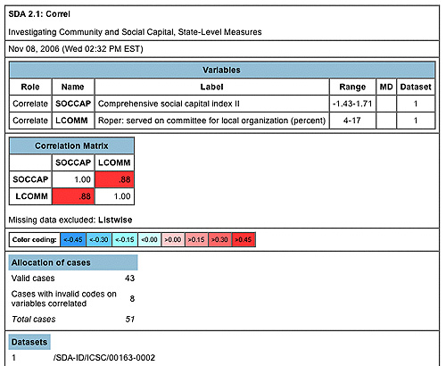
Let’s interpret these results.
The colored area reveals that the correlation between the social capital index and “served on a committee of local organization in last year” is .88 (the largest value a correlation can take on is 1.0 or -1.0). The results reveal that “served on a committee of local organization in last year” has a higher correlation with the social capital index than many of the variables (except for trust) in table 4.
However, notice that all the variables in table 4 have correlations of .65 or higher. Because of these higher numbers, Putnam argues that all these variables “fit together” well. He writes on page 291, “These fourteen indicators of formal and informal community networks and social trust are in turn sufficiently intercorrelated that they appear to tap a single underlying dimension.” Overall, in order to argue that variables can be “fit together” into a single index, such as the social capital index, they need to be sufficiently interrelated to each other. One way to examine this is to run a correlation matrix. You can do this with variables that measure traits other than social capital as well. What variables in this dataset might be used to create a “political participation index” for the fifty states?
Figure 80 on page 293 of Bowling Alone presents a geographic “portrait” of levels of social capital in the fifty states, based upon Putnam’s social capital index.
Open the state-level dataset and run a frequency on the social capital index (soccap) and examine the results as depicted in the image below.
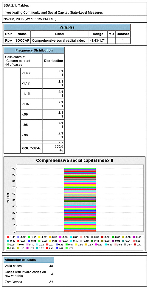
What do these numbers mean? First and foremost, the higher the number, the higher the level of social capital in the state. For example, the lowest social capital score is -1.43. What state is this? You can find out if you go back to the SDA analysis window and select “List values of individual cases” and “Start.” In the window that appears type in both “state” and “soccap” under the “Variables to List.” Your results will look like these shown in the image below:
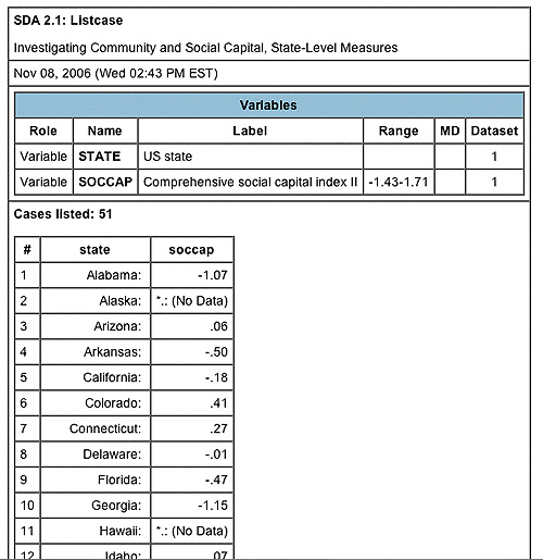
If you scroll down in the results, you will see that Nevada has the unusually low score of -1.43.
However, this still begs the question as to what the actual number -1.43 represents. Here is where it gets complicated. In order to create the social capital index, Putnam combines numerous variables that reflect the various components of social capital, such as political and civic participation and trust. Specifically, he uses the fourteen variables listed in Table 4 on page 291. However, most of these variables are measured on different scales. In order to combine them into one index, they must be “standardized” or placed on comparable scales. To do this, Putnam computed the standard score or z-score for each of these variables. Then, to compute an overall comprehensive social capital index score for each of the fifty states, he took the average of the standard scores for all the fourteen variables. This produces an average standard score for each of the fifty states in the dataset. This “score” takes on a small number that is negative or positive, because it has been “converted” to the scale of standard scores. And this is why the values in the frequency you produced above look a bit unusual at first glance.
If you are still confused, it will help to replicate what Putnam did. Open the state-level dataset and run a frequency, including summary statistics, on all the fourteen variables in Table 4 on page 291. If you do not remember how to do this, see Exercise 1 on this website.
A standard score or z-score is simply the deviation from the mean, divided by the standard deviation. In the frequencies you produced above, you have produced both the mean and the standard deviation for all fourteen variables. Save and/or print out these results so you can reference them as you continue with your analysis.
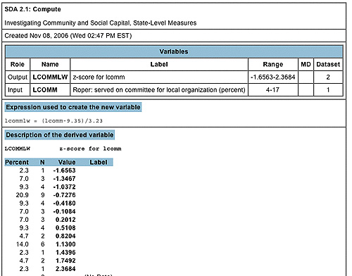
Now, let’s produce a standard score for “served on committee of local organization in last year” or “lcomm.” Return to the SDA analysis window for the state-level dataset with your browser’s “back” button. In the SDA analysis window, select “Compute a new variable” and “Start.” As depicted below, decide what unique name you will name your new variable (Just like recoding, consider adding your initials. I added mine to make “lcommlw”). Then type the equal sign and “(lcomm-9.35)/3.23” into the “EXPRESSION TO DEFINE NEW VARIABLE” box. This compute command is telling the computer to take “lcomm” and subtract it from the mean of 9.35 and divide by the standard deviation of 3.23. Under the “OPTIONAL” area, type “z-score for lcomm” into the “Label” box as shown in the image below.
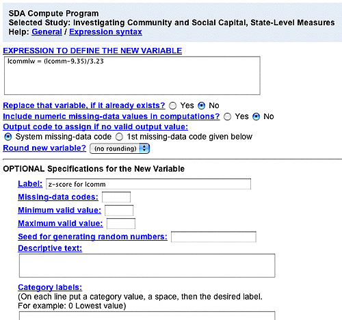
Once you select “Start computing,” a new screen will appear revealing that the values for “lcomm” have been converted to z-scores that range from -1.6563 to 2.3684. Your results should look like those shown in the image below:
Repeat this procedure for the remaining thirteen variables, and do not forget the names of each of your fourteen new variables. This is tedious, but replication will help you to more thoroughly understand how the index was created.
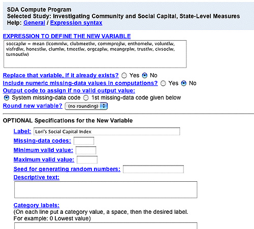
Once you have computed your fourteen new variables, you are now ready to take their average. Return to the SDA analysis window and select “Compute a new variable.” In the “EXPRESSION TO DEFINE NEW VARIABLE” box, type the name you choose to give to your social capital index and the equal sign. After the equal sign, type “mean( ).” Between the parentheses, type your fourteen new variable names, each separated by a comma. Do not forget to type a label for this variable. See the example below (note that your variable names will be different, since the names below contain my initials). Once you think you have got it, select “Start computing.”
Now answer Question 6.
In chapters 17-22, Putnam’s social capital index reveals some important relationships between the social capital index and other indicators of education, children’s welfare, safe and productive neighborhoods, economic prosperity, health and happiness, and democracy. To illustrate these relationships, Putnam provides numerous figures called scatterplots. Scatterplots provide a visualization of what is depicted numerically by the correlation coefficients that you produced earlier in this exercise.
On page 309, Figure 84 presents the “visual” correlation between social capital and murder rate in the fifty states. However, while SDA can produce bar charts and line charts in order to visualize your data, it cannot produce scatterplots. How can you replicate this scatterplot? To do this, you can export the data from SDA into the statistical programs, SPSS or Stata and produce a scatterplot using either of these software packages.
Open the state-level dataset and select “Download existing dataset and documentation” and “Start.” The following screen will appear.
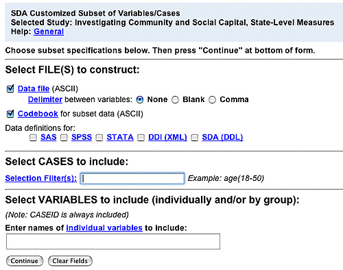
Select either the SPSS or Stata downloads. You are now ready to continue analysis of social capital data in either of these statistical programs, if your instructor wishes you to do so. However, for purposes of your investigation on this website, answer Questions 7-8.