Exercise 3: Why?
Deepen your investigation. In chapters 10 thru 15 of Bowling Alone, Putnam provides explanatory factors to help answer the question:
- Why has community declined in America?
On page 187 of chapter 10, Putnam writes, “The mysterious disengagement of the last third of a century has afflicted all echelons of our society.” Next, Putnam provides a long list of possible explanatory factors for the “crime” of disengagement–explanatory factors from which independent variables will be worked out in the ensuing chapters. This list is so long that Putnam then writes, “Most respectable mystery writers would hesitate to tally up this many plausible suspects, no matter how energetic their detective. . . . but we must begin to winnow the list.”
This exercise will introduce you to the difference between cross-sectional analysis and analysis over time. It will also introduce you to the idea of testing hypotheses using quantitative data. Finally, this exercise will teach you how to run and interpret crosstabulations in SDA.
A. Reading
- Read Bowling Alone, Chapters 10-15
- Questions 1-3
B. Running and Interpreting Crosstabulations With Two Variables
- Learn how to run and interpret crosstabulations with two variables
- Practice running a crosstabulation on “Did volunteer work” (volunt) and “Size of city residence” (citysize)
- Questions 4-5
C. Crosstabulations With a Third Control Variable
Questions
- According to Putnam in chapter 10, what are the several tests that explanatory factors must pass to assess their relative importance?
- Briefly discuss the qualifications that Putnam makes with regard to the conclusions about women’s employment/work and civic engagement.
- According to Putnam, what has been the single most important explanatory factor or prime suspect contributing to the decline in civic engagement? What is the second most important explanatory factor or suspect? Briefly explain why.
- In your crosstabulation on “Did volunteer work” (volunt) and “Size of city residence” (citysize), what are the percent differences between rural dwellers and the largest city dwellers?
- Compare your results in this crosstabulation with Putnam’s results in figure 50 on page 206. What is different or similar about doing volunteer work and serving as an officer or attending public meetings?
- In your crosstabulation on “Did volunteer work” (volunt) and “Size of city residence” (citysize), with “Work status” (emplmrg3) as a control variable, does work status appear to affect the original relationship? Why or why not? Be sure to discuss differences between categories of the independent variable, city size.
- Overall in chapter 12, does Putnam conclude that urbanization is a prime suspect or not? Why or why not?
Instructions and tutorials associated with this exercise
In Exercise 2, you focused your investigation on what has happened to civic engagement over time by examining and producing line graphs. You might have noticed that in order to do this, you always entered the “year” variable next to the “column” box in the SDA analysis window.
For this part of your investigation, you will be considering the “suspects” that may have lead to the “crime” of civic disengagement. Your detective work is about to get a bit more complicated since, instead of looking at what has happened to a single variable over time, you will be examining relationships between two or more variables. In other words, you will be exploring hypotheses , whereby the potential “suspects” are the independent variables, and the variables that reflect the “crime” of civic disengagement are the dependent variables.
Social scientists use many different statistical procedures to investigate hypotheses. The kind of data an investigator is analyzing usually guides what procedure is utilized. For your investigation, you will now be examining data that is either a nominal or ordinal level of measurement. A good way to investigate hypotheses in this kind of data is by using a procedure called crosstabulations, sometimes referred to as contingency tables.
Let’s begin crosstabulating.
For this exercise, instead of entering “year” in the column in the SDA analysis window, you will enter a potential “suspect”–the size of city residence. On page 205 in chapter 12, Putnam writes,
Compared with other Americans, residents of the nation’s largest metropolitan areas (both central cities and their suburbs) report 10-15 percent fewer group memberships, attend 10-15 percent fewer club meetings, attend church about 10-20 percent less frequently, and are 30-40 percent less likely to serve as officers or committee members of local organizations or to attend public meetings on local affairs. (Figure 50 and figure 51 illustrate these differences.)
Let’s produce something similar to figure 50 on page 206. However instead of exploring the hypothesis that city size affects both serving as an officer and attending public meetings, you will be exploring the hypothesis that city size affects working on a community project.
Open1 the DDB dataset. Again, you will be investigating the relationship between the “Size of city residence” (citysize) and “Worked on a community project” (commproj). However, before you can run your crosstabulation, you must recode “commproj” so that it is simplified into a variable that has only the two codes below (return to Exercise 2 if you need to refresh your memory on how to recode):
- 0 = None (Change the old code from ‘1’ into ‘0’ to make more sense.)
- 1 = Worked on a community project in past twelve months (Change the old codes ‘2 thru 7’ into ‘1’.)
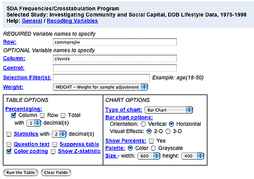
Once you have completed your recode, go back to the SDA analysis window and select “Run frequency or crosstabulation (with charts)” and type “your_unique_name” for your recoded variable after “Row” and type “citysize” after “Column” [instead of typing “year” like you did in Exercise 2]. Under “CHART OPTIONS” and “Type of chart,” select “bar chart” and under “Bar chart options” select the “horizontal” orientation. Finally, select “Run the Table” as shown in the image below.
As you can see below, your results look somewhat similar to figure 50 on page 206, with the exception that in SDA analysis the horizontal bar chart is inverted. The percentages appear on the top rather than the bottom of the chart. Consequently, rural towns appear on the top left, rather than the bottom left.
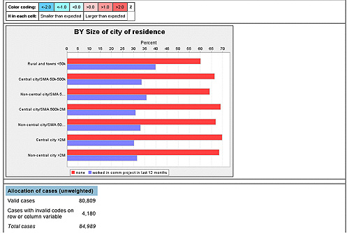
Now scroll up in your results window and examine the table that SDA has produced. Your results should match those depicted in the screen capture below.
Now, let’s interpret this table.
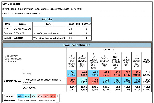
The first thing to note about this table is that the very bottom row contains “COL TOTAL” or column totals. You see 100 percent totals in each column because in SDA analysis, the default for percentages is the column. This is important because it assumes that you have entered your independent variable (the “suspect” of city size in this case) in the column. When investigating relationships with crosstabulations, it is essential that you examine the percentages within the categories of the independent variable. In this case, what is the difference between rural and urban dwellers in terms of working on a community project? Setting your table up the way the table above is set up, with the independent variable in the column, is a good practice to follow. This way you can train your investigative eye to look across–from left to right. Let’s try this with the table you produced.
Focus on the second row for those who worked on a community project (the first row is simply the “mirror” image, much like you saw in your line graphs for Exercise 2). Once you have focused your investigative eye on the second row, move it across from left to right, in order to examine the percentage differences across categories of the independent variable or the categories of city size. How big of a percentage difference is there between rural dwellers and the largest city dwellers? The answer: 39.9 percent compared to 31.6 percent, which is a 8.3 percent difference. If you compare this to figure 50 on page 206, you can see that the percentage differences are a bit larger in figure 50 compared to your analysis with community projects as your dependent variable. This is not surprising, given that serving as officers and attending public meetings are civic activities that require even more engagement than working on a community project, and consequently one might expect even larger differences between rural and city dwellers.
There is, however, one more important thing to note about the table you produced. It does not compare differences across time. Instead, you are looking at the totals for all the surveys conducted by the DDB from 1975 to 1998. Each survey that the DDB conducted, from 1975 to 1998, represents a “snapshot” in time, much like taking a picture. The technical term for this in survey research is a “cross-section.”
- Is it possible that the differences between rural and city dwellers has become more pronounced over time?
To investigate this, let’s compare two snapshots or cross-sections of time–1975 and 1998.
Open online analysis in new window the DDB dataset. Run a crosstabulation between “Size of city residence” (citysize) and your recoded variable for “Worked on a community project,” but before you run the table type “year(1975)” in the “Selections Filter(s)” box. Under “CHART OPTIONS” and “Type of chart,” select “bar chart” and under “Bar chart options” select the “horizontal” orientation.
- What are the percentage differences in this table between rural and city dwellers?
Run the same crosstabulation for 1998 and compare your results with 1975. Your investigation will reveal that a similar relationship existed in 1975 and 1998. City life, even in 1975, leads to less engaged citizens. This analysis reveals, so far, that urbanization may not be the prime suspect. But the story is more complicated than this. There are a lot of other potential suspects or explanatory factors for civic disengagement. Some of these factors may be tangled up with urbanization, something like “accessories” to a crime. Return to Exercise 3 to learn about controlling for other suspects.
Your crosstabulations in the last tutorial revealed that city size is a potential “suspect.” However, there are a lot of other potential “suspects” or explanatory factors for civic disengagement. These additional suspects can complicate social science investigation. Was civic disengagement due to something else? On the bottom of page 205-206, Putnam writes, “Could it be that the type of people who congregate in the biggest metropolitan areas are somehow predisposed against civic engagement? To rule this out, we reexamined the evidence, simultaneously holding constant a wide range of individual characteristics–age, gender, education, race, marital status, job status, parental status, financial circumstances, home ownership, region of the country.”
When Putnam refers to “holding constant” in the quote above, he is referring to the idea of scientific control. You are likely to be somewhat familiar with the idea of scientific control , which conjures up the image of a scientist working in a laboratory with a white lab coat.
Scientists in the laboratory are able to isolate potential explanatory factors. Sometimes social science investigators are able to isolate factors as well using the experimental research method, but much of social science research takes place outside the laboratory–in the messy world of society where crimes also take place. Therefore, social science investigators collect as many potential suspects as they can in order to “rule them out” as possible explanations for what they are investigating. This is what Putnam does in chapters 10-15 of his book, Bowling Alone.
Overall, in order to “rule out” potential suspects, social science investigators often use procedures of control statistically, rather than through experiments. One statistical procedure used to do this is controlling for a third variable in a crosstabulation.
A lot of the graphics that Putnam uses in the book illustrate controlling for third variables. For example, figure 49 on page 200 illustrates the relationship between work status and club meeting attendance, holding constant or controlling for whether one works out of necessity or for satisfaction. As Putnam writes, “full-time work significantly depresses club attendance, regardless of whether work is a choice or a necessity.”
Let’s extend the crosstabulation that you produced on city size and working on a community project by controlling for homeownership, one of the characteristics that Putnam holds constant on page 206.
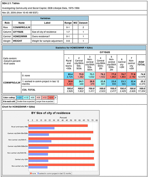
Open  the DDB dataset. Run a crosstabulation between “Size of city residence” (citysize) and your recoded variable for “Worked on a community project,” but before you run the table type “homeownr” in the “Control” box. Under “CHART OPTIONS” and “Type of chart,” select “bar chart” and under “Bar chart options” select the “horizontal” orientation. Finally, select “Run the Table.”
You will get a lot of results, since the control procedure produces a separate crosstabulation for each code that you have for your control variable. In the case of homeownership, there are two codes (0 = no, 1 = yes). Therefore, your results are two tables–one table is only people who do not own a home and the other table is only homeowners. In this way, it is clear how you are able to hold constant or control for the additional independent variable of homeownership.
Let’s interpret these results.
Examine the table for people who do not own a home.
- What is the percentage difference between rural dwellers and the largest city dwellers who worked on community projects? (30.6 percent compared to 22.4 percent, respectively, for a percent difference of 8.2)
Now, compare this percentage difference to the table for homeowners.
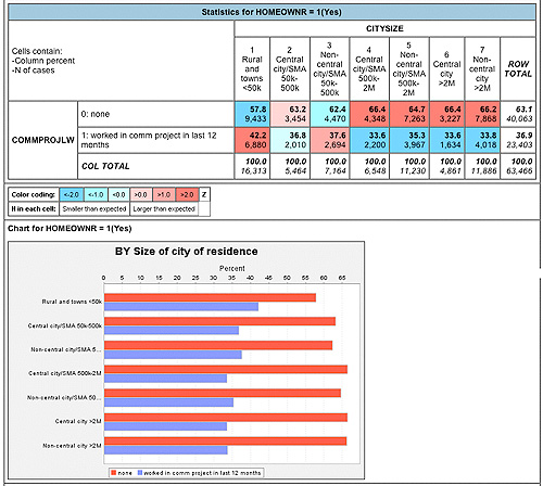
- Are homeowners different? (42.2 percent compared to 33.8 percent, respectively, for a percent difference of 8.4)
These results support Putnam’s conclusions that homeownership (and other characteristics) does not change the relationship between city size and civic engagement.
Return to Exercise 3 to practice producing and interpreting your own crosstabulation that controls for a third variable.