ICSC Exercise 1: Getting Started
Now it is time to formally begin your investigation. This exercise will introduce you to some of the quantitative social science evidence presented in Bowling Alone and teach you how to search codebooks, and how to run frequencies and summary statistics using SDA.
A. Reading
- Read Bowling Alone, Chapters 1-3
- Answer Questions 1-3
B. Searching Codebooks
- Learn how to search codebooks for variables
- Practice searching the DDB codebook for the variable “Went to a club meeting” (CLUBMEET)
- Answer Questions 4-5
C. Running and Interpreting Frequencies, Bar Charts, and Summary Statistics
Turn to the bottom of page 59 in Bowling Alone where Putnam writes, “In 1987, 61 percent of all organization members had served on a committee at some time or other, and 46 percent had served as an officer.” You can reproduce or replicate these percentages.
- Practice searching the GSS codebook for variables about serving on a committee and as an officer. To do this, follow the same logic that you learned above about searching the DDB codebook.
- Learn how to run and interpret frequencies
- Practice running a frequency on “Has R served as officer in group?” (LEADGRP)
- Answer Questions 6-7
On page 60, Putnam writes “In twenty-five annual surveys between 1975 and 1999 the DDB Needham Lifestyle surveys asked more than eighty-seven thousand Americans ‘How many times in the last year did you attend a club meeting?’”
- Practice searching the DDB codebook for this variable and running a frequency on this variable
- Learn how to run and interpret a frequency and summary statistics on club meeting attendance for 1987
- Practice running a frequency on club meeting attendance for a year other than 1987
- Answer Questions 8-9
Questions
- Discuss the difference between “bridging” and “bonding” social capital.
- What is intercohort versus intracohort change? Discuss this in relation to what has happened to political and civic participation over the last quarter of the twentieth century.
- What has happened to the number of nonprofits between 1968 and 1997? Is this a useful indicator or “barometer” of civic participation, according to Putnam? Why or why not? What about official membership in formal organizations?
- What do the codes of ‘1’ and ‘2’ represent for the variable “clubmeet?”
- What is another variable in the DDB dataset, like “clubmeet,” that is about civic engagement?
- How is “SERVEGRP” coded and what is the level of measurement? Explain why it is this level of measurement.
- What does the frequency of those who have served as group officers in 1987 reveal about what Putnam calls “active participation?” What happens it the next decade, according to Putnam? What evidence does he provide for this?
- In the frequency for “clubmeet” for a year other than 1987, briefly explain your results, including the bar graph.
- In the frequency for “clubmeet” for a year other than 1987, explain the following summary statistics: mode, median, mean, range, variance and standard deviation.
Instructions and tutorials associated with this exercise
If you were looking at a “raw” dataset, all you would see are rows and columns of numbers called a “data matrix.” There are several ways to makes sense of a data matrix. First, statistical packages (e.g., SPSS and Stata) and spreadsheet programs (e.g., Excel) often contain labels for what each column represents in a data matrix. In the datasets you will be using for your investigation, each column of numbers represents a variable, and each row of numbers represents a “case” in the data, which is another term for the unit of analysis.
For example, in the DDB dataset, the unit of analysis is individuals. Therefore, if you were looking at the raw dataset, there would be exactly 84,989 rows. Why so big? If you remember, the DDB Needham marketing company conducted surveys of 3,500-4,000 individuals from the year 1975, and the dataset for your investigation goes through 1998.
However, what is unique about using the SDA Web-based software is that you never actually see the raw dataset. The next best way to make sense of it is to look at a codebook. A codebook is like a guidebook for datasets. One of its most important functions is to provide details about each variable in the dataset.
Let’s look at an example using the DDB data.
When you first open the DDB dataset, you will see the Authorized Download window where you have to first log on to your account at the ICPSR data archive at the University of Michigan (if you have not already created an account, you can do so now).
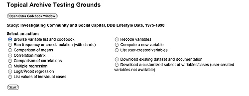
Once you have logged on, the following window will appear where you can select Open Extra Codebook Window at the top:
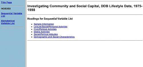
Another window will open that will allow you to select from the three search options under Indexes. Select the Sequential Variable List. Once you do this, a window will appear with the following groupings for the DDB dataset: Sample Information, Leisure/Social/Personal Activities, Civic/Political Activities, Media Activities, Social and Political Attitudes, and Demographic and Social Characteristics.
On the left hand side is the shorthand variable name with a brief description of the variable immediately following. For example, under Leisure/Social/Personal Activities the variable “beerbar” is the shorthand name for the variable “Went to a bar or tavern (freq last 12 months).” This is not the most detailed description possible, since the best detail would be the exact question wording. However, for the DDB data, this is all that we have and it is sufficient for our investigation.
If you select “beerbar,” a window showing the frequency of the variable will appear.
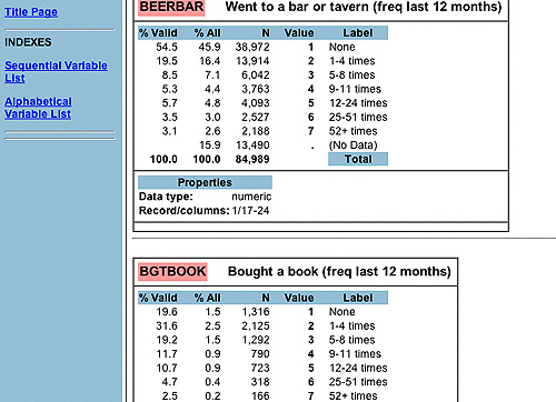
This frequency reveals even more information about the variable, for example, a ‘1’ means that an individual in the survey did not go to a bar or tavern in the last 12 months. In addition to what the codes such as ‘1’ represent, there is a lot more information packed into this frequency that you will learn about next in Exercise 1.
In the practice you just completed, you should have found the variable names for the variables in the General Social Survey about serving on a committee and as an officer: “SERVEGRP” and “LEADGRP.” You should have also noticed that searching in the General Social Survey follows a similar logic to searching in the DDB data, even though the former contains a lot more variables.
You also learned that if you select the variable name in the codebook window, it shows more detailed information. This information is called a frequency distribution . At this point you should consult your favorite statistics book about frequencies and, in addition, familiarize yourself with an important companion concept: level of measurement .
Rather than relying upon the frequency already produced for you in the codebook, there is a preferable way to run frequencies yourself, which gives you more investigative power.
Let’s look at an example for running a frequency on SERVEGRP or “Has R [respondent to the survey] served on group committees.”
After you open the General Social Survey SDA dataset and select “Frequencies or crosstabulation (with chart)” and the “Start” button, the following screen will appear where you can type “SERVEGRP” next to “Row.” In addition, SDA allows you to create special types of bar graphs to better visualize your results. For this example, under “CHART OPTIONS” select the “Bar Chart” option next to “Type of charts.”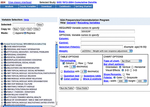
Next select the Run the Table button at the bottom of the screen and obtain the results.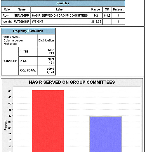
Let’s interpet these results.
The first thing you should notice is that a code of ‘1’ means that an individual has served on group committees and ‘2’ means that an individual has not. This coding reveals that the variable “SERVEGRP” is measured at the nominal level of measurement .
Most important, the frequency reveals that a healthy 60.7 percent of the sample surveyed has been engaged in civic life in this manner. Moreover, in the bar graph you can see how large 60.7 percent is compared to those who did not serve on a group committee. This simple visual representation (one can immediately see that there are more who answered “yes” than “no”) is often what makes graphs, charts, and tables a powerful way to communicate quantitative information. Visual representations of quantitative information often are underutilized (see Edward Tufte , a scholar who writes about this). In Bowling Alone, because Putnam writes for a more general audience, he pays particular attention to this, and hence presents a lot of the quantitative evidence visually.
On page 59 of Bowling Alone, Putnam rounds the figure 60.7 percent up to 61 percent. Also notice that this is just for the year 1987. If you read on to page 60, Putnam explains what happens in the next decade in America to this picture of what he calls “active participation,” and it is represented visually in Figure 10.
Before we move on, there is still more to learn from this frequency. How many individuals were surveyed? An exact 1,174 individuals answered this question on the survey. Why so small? Again, if you delve into the codebook a bit further, you will learn that the variable “SERVEGRP” only occurs in the year 1987, when the GSS conducted a special investigation into civic engagement. This is why Putnam has to use other datasets and variables to produce Figure 10 on page 60. But for now, congratulations are in order. You have been able to replicate some of Putnam’s work and apply knowledge about frequencies and level of measurement to your investigation. Now return to Exercise 1 to practice replicating Putnam’s reported frequency on serving as an officer in a group in 1987.
Since the DDB dataset includes annual surveys from 1975 to 1998, when you run a frequency, you will get the results for every year’s survey that included that particular variable, for a possible total of 84,989 individuals. It is important to notice that it will not always be clear which years are contained in the results because not all the variables were included every year’s survey. For example, the question about using automatic teller machines was not asked in the earlier DDB surveys because automatic tellers did not exist yet.
Because of this confusion and because each year is its own separate sample, when you are doing applied statistical analysis with data collected over numerous years like the DDB and the GSS, most of the time you should analyze the variables for a particular year (except when you are doing timelines and need to look at surveys over a number of years, but you will learn more about this in Exercise 2).
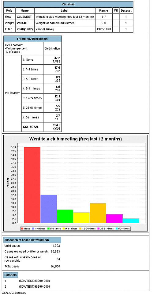
Let’s look at an example of how to run a frequency on club meeting attendance (clubmeet) for 1987.
Open the DDB dataset, select “Frequencies or crosstabulation (with charts),” and select the “Start” button. An analysis window like the one below will appear. Type “clubmeet” next to “Row” and next to “Selection Filter(s)” type “year(1987).” In addition, under “CHART OPTIONS” select the “Bar Chart” option next to “Type of chart.”

After you “Run the Table” you will get the following results. Note that the total number of individuals for the 1987 survey was 4,003 and that 1,889 individuals or 47.2 percent of the sample did not attend a club meeting in the last 12 months. Also note that there are a lot more “codes” in this frequency distribution than the one you did for served on a group committee in the last tutorial. Instead of a simple “yes” or “no” answer, this variable asks a person to provide more numerical detail about their activity. This type of ordered variable is an example of the ordinal level of measurement . Be sure to be a conduct a thorough investigation and consult your statistics/methods book about level of measurement.
So far you have acquired several investigative skills:
- Searching Codebooks
- Running and Interpreting Frequencies
To wrap up your investigation in Exercise 1, you still need the following:
- Running and Interpreting Summary Statistics
Let’s look at one more example with club meeting attendance (clubmeet) for 1987.
Open the DDB dataset and run the frequency for “clubmeet” in 1987 like you did above, except before you select “Run the Table,” be sure to check “Statistics” under the “TABLE OPTIONS.” Do not forget to type “year(1987)” next to “Selection Filter(s)” and to select the “Bar Chart” option. Now you can “Run the Table” to produce the following:
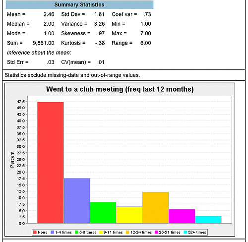
Let’s interpret these results:
Your frequency distribution can be interpreted similarly to what you did above. Except in these results, you also have some additional information under “Summary Statistics.” There are fourteen different statistics here. Not to worry; you do not have to know about all of them for the introductory level. First, let’s focus on the mode , median , and mean or “measures of central tendency.” Again, be a thorough investigator and consult your statistics/methods book.
The mean of 2.46 is slightly higher than the median of 2.00 (the mean is getting pulled up by those super active people who attend a lot of meetings). But the ordinal level of measurement is not super precise so the median, or the whole number “2,” makes a lot more sense to interpret here (why?). The median of 2.00 represents the category of “1-4 times.” This is the middle or the center of the frequency distribution. What does this tell us? Basically, not very many people in 1987 are going to very many club meetings, because half of the people are below this in the category of “None.” In fact the mode is “1,” attending no meetings in the past 12 months. The fact that 47.2 percent, or nearly half of the people surveyed did not attend a club meeting begins to build support for Putnam’s claim in Chapter 3–although the number of associations may have been on the rise and large numbers of people claimed membership in these associations, not many people are “active” participants. Keep in mind, however, that your statistics here are only for a particular year. What has happened over time? You will get to explore this with timelines in Exercise 2.
Now let’s focus on three other introductory summary statistics: the range , variance , and standard deviation , or “measures of variability/dispersion.” The range for this variable is 6.00. This tells us that there were a variety of codes for this variable, or 7.00 -1.00 = 6.00. Therefore, because of how the question was asked, there is more room for variability. You might understand this better if you think of the analogy of answering true/false questions as opposed to multiple choice on an exam. An instructor is going to get more variability in test scores on a multiple choice exam.
The variance and standard deviation can be interpreted together, since the standard deviation is simply the square root of the variance. For interpreting the “clubmeet” frequency distribution, the variance and standard deviation are not really all that applicable, because this variable is an ordinal level of measurement. Variance and standard deviation are used, in the strict sense, for interval level variables. However, sometimes it is okay to “bend the rules,” so let’s look at the standard deviation in this situation because there are 7 categories and more variability is possible, just like a multiple choice exam.
A standard deviation of 1.81 is very close to 2.00. So the best way to interpret it is to say that, on average, most people fall between 2.00 categories above and below the mean of 2.46 (round to 2.00). This means that most people are between the codes of “1” and “4” or not attending meetings and attending 9-11 times. The response of 9-11 times is 2.00 above the mean of 1-4 times, and “None” is as far below the mean as is possible. Now you can see why it is so important to have a codebook and to know what the numbers represents, especially in the DDB data where a “1” means “None.” This also shows why it is so important when conducting investigation that it is important to be meticulous. A crime scene investigator has to be meticulous as well, since tainted evidence does not hold up well in the courtroom. Now return to Exercise 1 and practice your ability to be meticulous by running summary statistics on club meeting attendance for a year other than 1987.